How do you choose between Poisson and negative binomial models for discrete count outcomes?
One key criterion is the relative value of the variance to the mean after accounting for the effect of the predictors. A previous article discussed the concept of a variance that is larger than the model assumes: overdispersion.
(Underdispersion is also possible, but much less common).
There are two ways to check for overdispersion:
- The Pearson Chi2 dispersion statistic
The Pearson Chi2 dispersion statistic for the model run in that article was 2.94. If the variance is equal to the mean, the dispersion statistic would equal one.
When the dispersion statistic is close to one, a Poisson model fits. If it is larger than one, a negative binomial model fits better.
- Residual Plots
Plotting the standardized deviance residuals to the predicted counts is another method of determining which model, Poisson or negative binomial, is a better fit for the data.
Here is the plot using a Poisson model when regressing the number of visits to the doctor in a two week period on gender, income and health status.
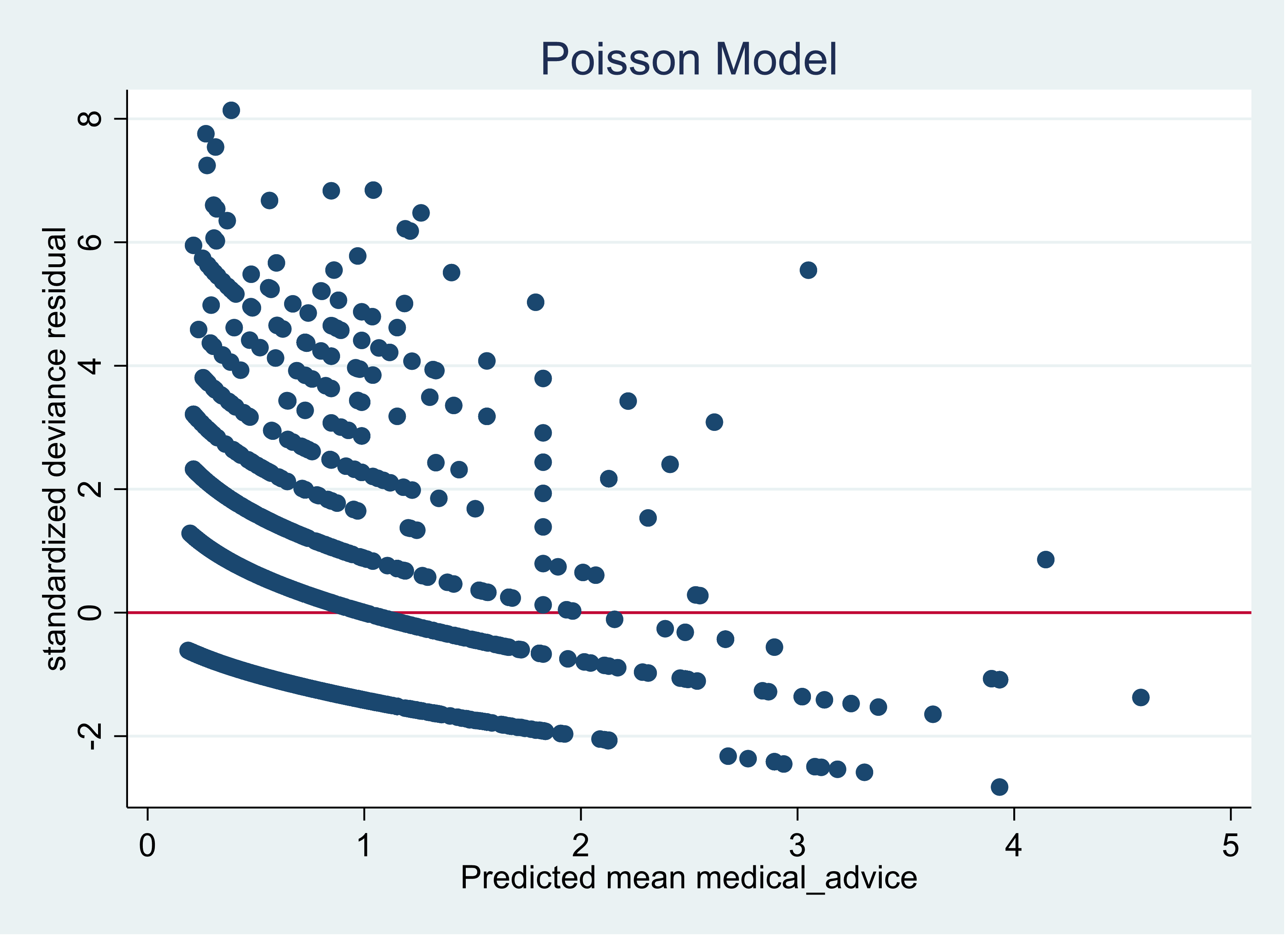
The series of waves in the graph is not an unusual structure when graphing count model residuals and predicted outcomes.
Our primary focus is on the scale of the y axis. A good fitting model will have the majority of the points between negative 2 and positive 2. There should be few points below negative 3 and above positive 3.
Adding more predictors to the model can have an impact on improving the plot but the Poisson model is clearly a very poor fitting model for these data.
If we use the same predictors but use a negative binomial model, the graph improves significantly.
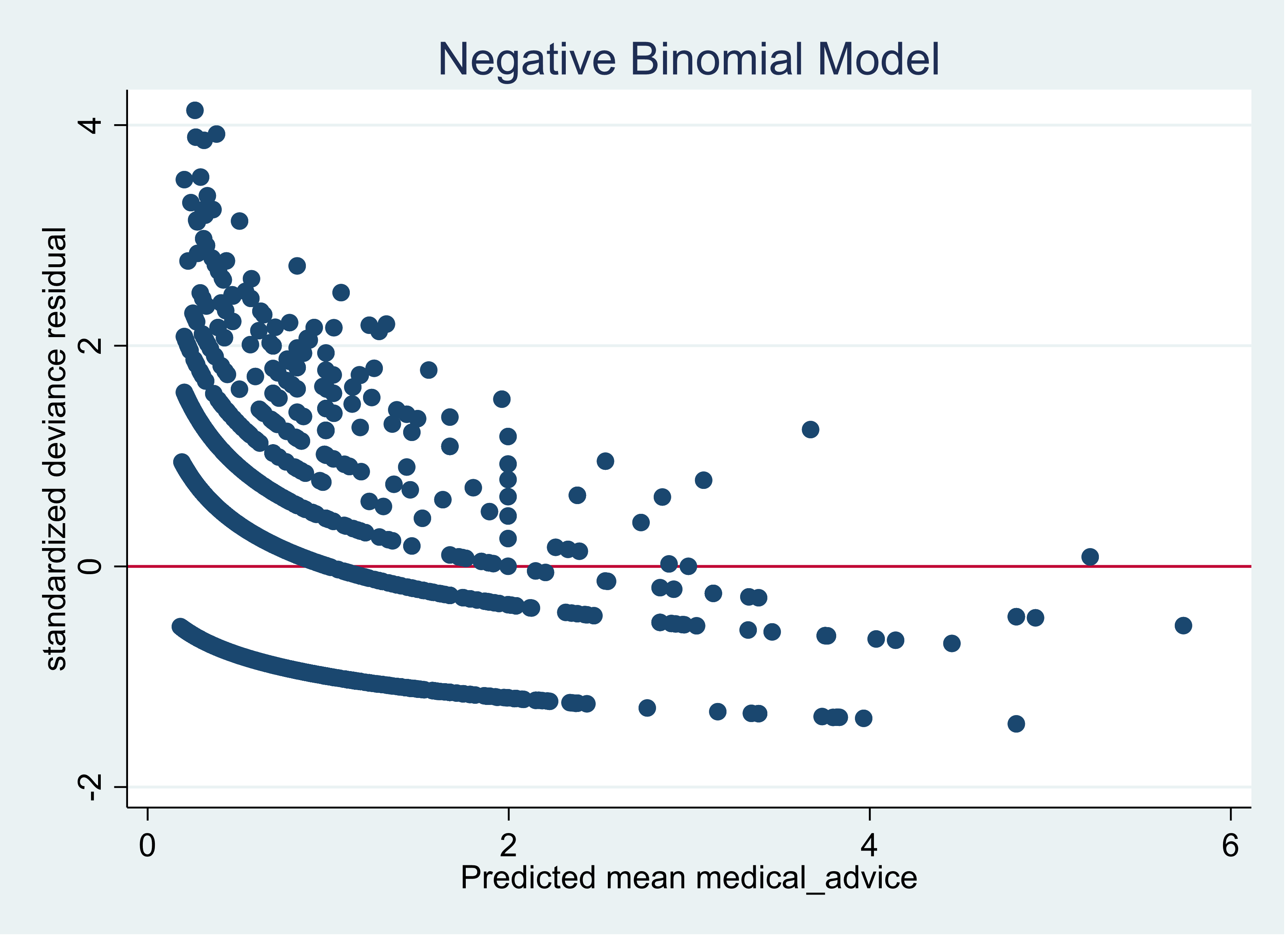
Notice now the maximum value for the standardized deviance residual is now 4 as compared to 8 for the Poisson model. The model still has room for improvement. That would require, if they are available, selecting better predictors of the outcome.
Now let’s compare the graphs when the Pearson Chi2 dispersion is closer to one. We will now regress the count of rabbits per 400 square yard plots on shrub coverage, density of shrubbery and variety of shrubbery. The Pearson Chi2 dispersion for this model is 1.15.
Using a Poisson model our graph looks like this:
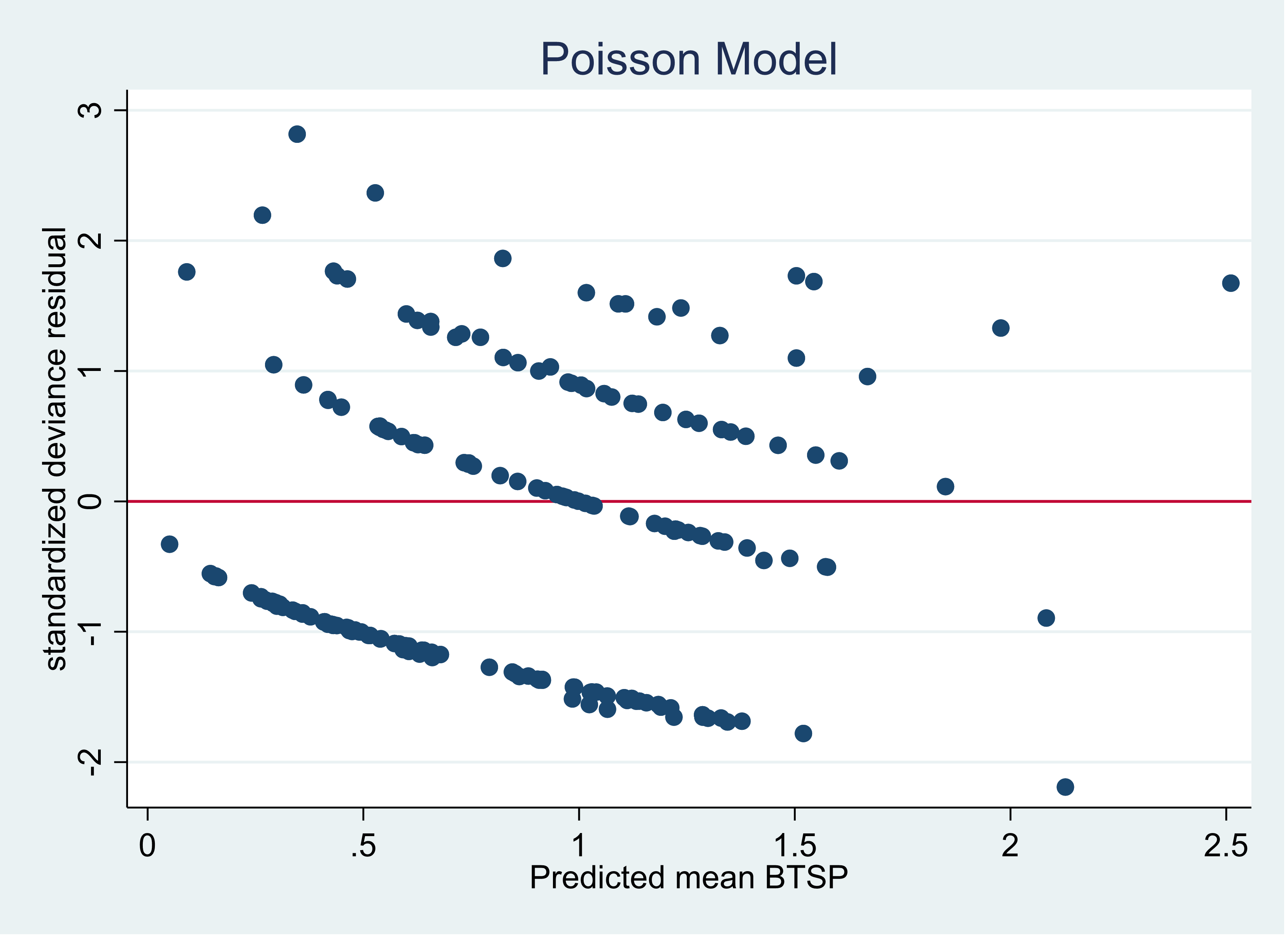
Almost all of the residual points are now inside of negative 2 and positive 2.
Here is the graph of the negative binomial model using the same predictors:
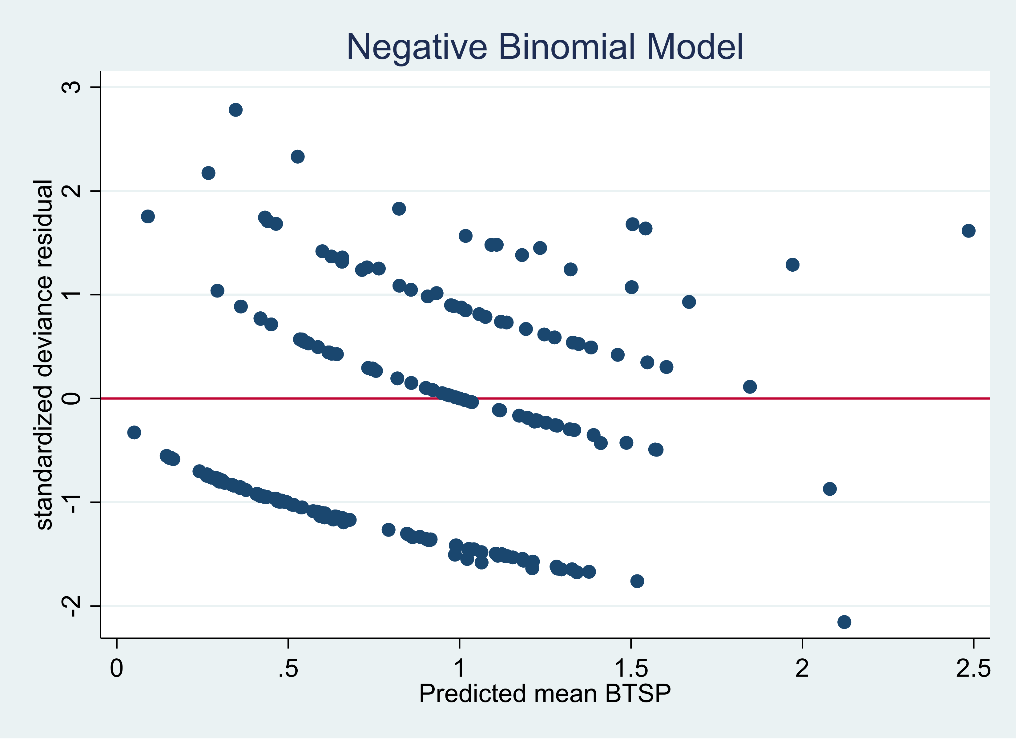
The two graphs are nearly identical.
As you have seen, graphing the standardized deviance residuals by the predicted outcomes can help us verify which type of model is a better fit for your data.
Jeff Meyer is a statistical consultant with The Analysis Factor, a stats mentor for Statistically Speaking membership, and a workshop instructor. Read more about Jeff here.

I found this very useful. The discussion on graph interpretation was exactly guidance I was looking for.
My question is the same as the first comment.
How do you calculate standardised deviance residuals?
I am using r-code and I have googled for an answer on this with no success.
Hi,
This is an example for the code for a model:
model_nb <- glm.nb(medical_advice ~ sex + age_cen + income +
hscore + nonpresc , data=adv, control = glm.control(maxit = 100))
To generate the deviance residual:
dev_std_nb<-rstandard(model_nb)
how to calculate standardize deviance residual manually ? I try to use it in python
Hi, thanks a lot for this interesting article? What are the commands for the residual plots?
Thanks for your kindest support
I created the graphs using Stata. First you generate the residuals and the linear predicted values.
predict dev_nb, deviance standard // deviance residual
predict xb_nb, xb //linear prediction
The qnorm plot:
qnorm dev_nb, title (“negative binomial”)
Scatter plot
twoway(scatter dev_nb xb_nb)
Jeff
Hi Jeff,
Thnaks a lot for this.
These commands are not working with my STATA.
Could you please explain
Hello:
I have a question regarding this as well: how would you test for over dispersion in GAMMs? I have data that I believe is zero-inflated but I want to check whether to apply a negative binomial or a poisson would be better?
I’m very new with these types of statistics and have found myself very confused.
Thank you!
Hi Kelsey,
It’s my view that “zero inflated” is a misleading term. It actually does not mean that you have a lot of zeros in your outcome variable. Zero inflated means you have observations in your data set that can only be zeros. For example, let’s suppose your outcome is “number of fish caught” by people on the pier. There might be people on the pier that aren’t trying to catch fish, they might be there to enjoy the smell of the salt in the air. People not fishing would be considered to be zero inflated and should be accounted for differently.
Regarding how do you determine whether you should use a negative binomial model or a Poisson model, my first choice is to use a negative binomial model. If the data is not overdispersed the negative binomial model will most likely not converge. If it doesn’t converge I would then use a Poisson model.
Jeff
Hello:
I had a question. On this page you stated that a good fitting model would have the majority of its residual points between 2 and -2. I am wondering why this is the case? Any help you could provide would be fantastic.
Hi Benjamin,
Our goal for a good fitting model is a normal distribution of our residuals. In a standardized normal distribution (think of the bell curve) approximately 95% of all of the observations are between -2 and +2. We would like to see that pattern with our standardized residuals. In the case for count models with discrete outcomes, we use the standardized deviance residuals because they have been modified to reflect the distribution that we would have with a continuous outcome. Standardized Pearson residuals should not be used.
Jeff