Data Preparation

From our last article, you should feel comfortable with the idea of editing and saving data sets in Stata. In this article, we’ll explain how to create new variables in Stata using replace, generate, egen, and clonevar.

(more…)

No comments yet

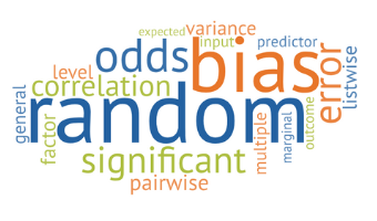Level is a statistical term that is confusing because it has multiple meanings in different contexts (much like alpha and beta).

There are three different uses of the term Level in statistics that mean completely different things. What makes this especially confusing is that all three of them can be used in the exact same analysis context.

I’ll show you an example of that at the end.

So when you’re talking to someone who is learning statistics or who happens to be thinking of that term in a different context, this gets especially confusing.

Levels of Measurement

The most widespread of these is levels of measurement. Stanley Stevens came up with this taxonomy of assigning numerals to variables in the 1940s. You probably learned about them in your Intro Stats course: the nominal, ordinal, interval, and ratio levels.

Levels of measurement is really a measurement concept, not a statistical one. It refers to how much and the type of information a variable contains. Does it indicate an unordered category, a quantity with a zero point, etc?

So if you hear the following phrases, you’ll know that we’re using the term level to mean measurement level:

• nominal level
• ordinal level
• interval level
• ratio level

It is important in statistics because it has a big impact on which statistics are appropriate for any given variable. For example, you would not do the same test of association between two variables measured at a nominal level as you would between two variables measured at an interval level.

That said, levels of measurement aren’t the only information you need about a variable’s measurement. There is, of course, a lot more nuance.

Levels of a Factor

Another common usage of the term level is within experimental design and analysis. And this is for the levels of a factor. Although Factor itself has multiple meanings in statistics, here we are talking about a categorical independent variable.

In experimental design, the predictor variables (also often called Independent Variables) are generally categorical and nominal. They represent different experimental conditions, like treatment and control conditions.

Each of these categorical conditions is called a level.

Here are a few examples:

• In an agricultural study, a fertilizer treatment variable has three levels: Organic fertilizer (composted manure); High concentration of chemical fertilizer; low concentration of chemical fertilizer.So you’ll hear things like: “we compared the high concentration level to the control level.”
• In a medical study, a drug treatment has three levels: Placebo; standard drug for this disease; new drug for this disease.
• In a linguistics study, a word frequency variable has two levels: high frequency words; low frequency words.

Now, you may have noticed that some of these examples actually indicate a high or low level of something. I’m pretty sure that’s where this word usage came from. But you’ll see it used for all sorts of variables, even when they’re not high or low.

Although this use of level is very widespread, I try to avoid it personally. Instead I use the word “value” or “category” both of which are accurate, but without other meanings. That said, “level” is pretty entrenched in this context.

Level in Multilevel Models or Multilevel Data

A completely different use of the term is in the context of multilevel models. Multilevel models is a 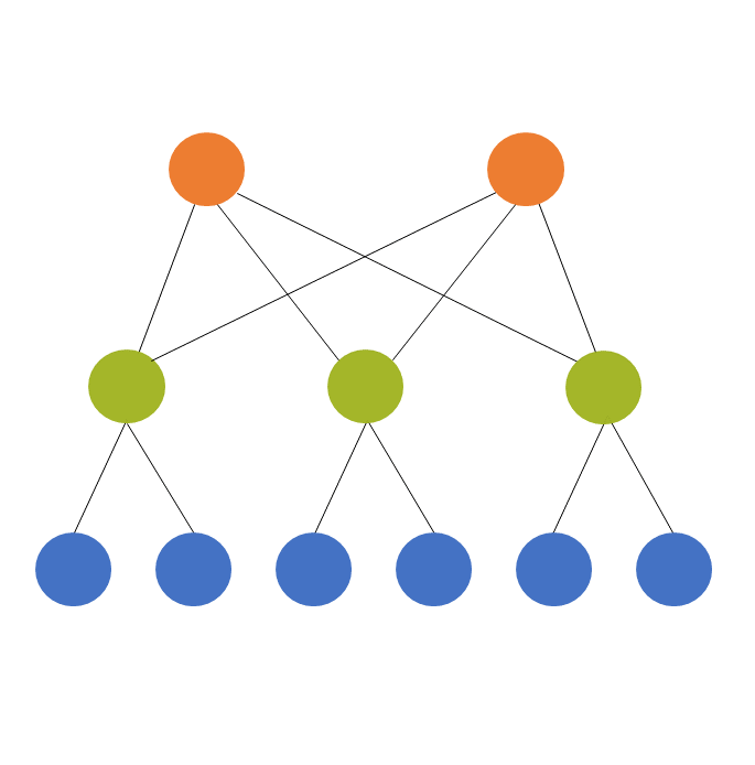term for some mixed models. (The terms multilevel models and mixed models are often used interchangably, though mixed model is a bit more flexible).

Multilevel models are used for multilevel (also called hierarchical or nested) data, which is where they get their name. The idea is that the units we’ve sampled from the population aren’t independent of each other. They’re clustered in such a way that their responses will be more similar to each other within a cluster.

The models themselves have two or more sources of random variation.  A two level model has two sources of random variation and can have predictors at each level.

A common example is a model from a design where the response variable of interest is measured on students. It’s hard though, to sample students directly or to randomly assign them to treatments, since there is a natural clustering of students within schools.

So the resource-efficient way to do this research is to sample students within schools.

Predictors can be measured at the student level (eg. gender, SES, age) or the school level (enrollment, % who go on to college).  The dependent variable has variation from student to student (level 1) and from school to school (level 2).

We always count these levels from the bottom up. So if we have students clustered within classroom and classroom clustered within school and school clustered within district, we have:

• Level 1: Students
• Level 2: Classroom
• Level 3: School
• Level 4: District

So this use of the term level describes the design of the study, not the measurement of the variables or the categories of the factors.

Putting them together

So this is the truly unfortunate part. There are situations where all three definitions of level are relevant within the same statistical analysis context.

I find this unfortunate because I think using the same word to mean completely different things just confuses people. But here it is:

Picture that study in which students are clustered within school (a two-level design). Each school is assigned to use one of three math curricula (the independent variable, which happens to be categorical).

So, the variable “math curriculum” is a factor with three levels (ie, three categories).

Because those three categories of “math curriculum” are unordered, “math curriculum” has a nominal level of measurement.

And since “math curriculum” is assigned to each school, it is considered a level 2 variable in the two-level model.

See the rest of the Confusing Statistical Terms series.

First published December 12, 2008

Last Updated January 21, 2025

No comments yet

Once you’ve imported your data into Stata the next step is usually examining it.

Before you work on building a model or running any tests, you need to understand your data. Ask yourself these questions:

• Is every variable marked as the appropriate type?
• Are missing observations coded consistently and marked as missing?
• Do I want to exclude any variables or data points?

(more…)

No comments yet

SPSS has a nice little feature for adding and averaging variables with missing data that many people don’t know about.

It allows you to add or average variables that have some missing data, while specifying how many are allowed to be missing. (more…)

No comments yet

In our previous posts, we’ve relied on Stata’s pre-loaded datasets to perform analyses. But when you’re working with your own data, you’ll need to know how to import it into Stata.

To demonstrate how this process works, we will use the Iris dataset from UCI.

Download the dataset, then move it to whichever directory you intend to use for Stata files.

There are three main ways of importing data in Stata: either use the menus to import the data, call the dataset by its full file extension, or change your directory to the one with your data and then refer to the dataset by name. (more…)

No comments yet

(more…)

No comments yet