By Manolo Romero Escobar
What is a latent variable?
“The many, as we say, are seen but not known, and the ideas are known but not seen” (Plato, The Republic)
My favourite image to explain the relationship between latent and observed variables comes from the “Myth of the Cave” from Plato’s The Republic. In this myth a group of people are constrained to face a wall. The only things they see are shadows of objects that pass in front of a fire (more…)
One common reason for running Principal Component Analysis (PCA) or Factor Analysis (FA) is variable reduction.
In other words, you may start with a 10-item scale meant to measure something like Anxiety, which is difficult to accurately measure with a single question.
You could use all 10 items as individual variables in an analysis–perhaps as predictors in a regression model.
But you’d end up with a mess.
Not only would you have trouble interpreting all those coefficients, but you’re likely to have multicollinearity problems.
And most importantly, you’re not interested in the effect of each of those individual 10 items on your (more…)
A data set can contain indicator (dummy) variables, categorical variables and/or both. Initially, it all depends upon how the data is coded as to which variable type it is.
For example, a categorical variable like marital status could be coded in the data set as a single variable with 5 values: (more…)
One of the most confusing things about mixed models arises from the way it’s coded in most statistical software. Of the ones I’ve used, only HLM sets it up differently and so this doesn’t apply.
But for the rest of them—SPSS, SAS, R’s lme and lmer, and Stata, the basic syntax requires the same pieces of information.
1. The dependent variable
2. The predictor variables for which to calculate fixed effects and whether those (more…)
by Manolo Romero Escobar
General Linear Model (GLM) is a tool used to understand and analyse linear relationships among variables. It is an umbrella term for many techniques that are taught in most statistics courses: ANOVA, multiple regression, etc.
In its simplest form it describes the relationship between two variables, “y” (dependent variable, outcome, and so on) and “x” (independent variable, predictor, etc). These variables could be both categorical (how many?), both continuous (how much?) or one of each.
Moreover, there can be more than one variable on each side of the relationship. One convention is to use capital letters to refer to multiple variables. Thus Y would mean multiple dependent variables and X would mean multiple independent variables. The most known equation that represents a GLM is: (more…)
Fortunately there are some really, really smart people who use Stata. Yes I know, there are really, really smart people that use SAS and SPSS as well.
But unlike SAS and SPSS users, Stata users benefit from the contributions made by really, really smart people. How so? Is Stata an “open source” software package?
Technically a commercial software package (software you have to pay for) cannot be open source. Based on that definition Stata, SPSS and SAS are not open source. R is open source.
But, because I have a Stata license (once you have it, it never expires) I think of Stata as being open source. This is because Stata allows members of the Stata community to share their expertise.
There are countless commands written by very, very smart non-Stata employees that are available to all Stata users.
Practically all of these commands, which are free, can be downloaded from the SSC (Statistical Software Components) archive. The SSC archive is maintained by the Boston College Department of Economics. The website is: https://ideas.repec.org/s/boc/bocode.html
There are over three thousand commands available for downloading. Below I have highlighted three of the 185 that I have downloaded.
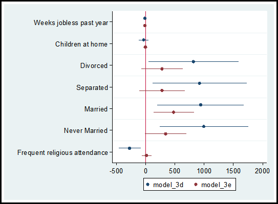
1. coefplot is a command written by Ben Jann of the Institute of Sociology, University of Bern, Bern, Switzerland. This command allows you to plot results from estimation commands.
In a recent post on diagnosing missing data, I ran two models comparing the observations that reported income versus the observations that did not report income, models 3d and 3e.
Using the coefplot command I can graphically compare the coefficients and confidence intervals for each independent variable used in the models.
The code and graph are:
coefplot model_3d model_3e, drop(_cons) xline(0)
Including the code xline(0) creates a vertical line at zero which quickly allows me to determine whether a confidence interval spans both positive and negative territory.
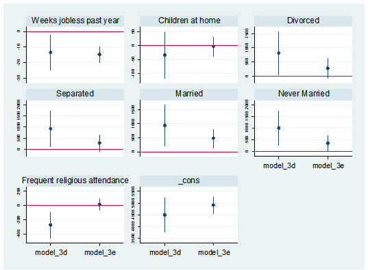
I can also separate the predictor variables into individual graphs:
coefplot model_3d || model_3e, yline(0) bycoefs vertical byopts(yrescale) ylabel(, labsize(vsmall))
2. Nicholas Cox of Durham University and Gary Longton of the Fred Hutchinson Cancer Research Center created the command distinct. This command generates a table with the count of distinct observations for each variable in the data set.
When getting to know a data set, it can be helpful to search for potential indicator, categorical and continuous variables. The distinct command along with its min(#) and max(#) options allows an easy search for variables that fit into these categories.
For example, to create a table of all variables with three to seven distinct observations I use the following code:
distinct, min(3) max(7)
In addition, the command generates the scalar r(ndistinct). In the workshop Managing Data and Optimizing Output in Stata, we used this scalar within a loop to create macros for continuous, categorical and indicator variables.
3. In a data set it is not uncommon to have outliers. There are primarily three options for dealing with outliers. We can keep them as they are, winsorize the observations (change their values), or delete them. Note, winsorizing and deleting observations can introduce statistical bias.
If you choose to winsorize your data I suggest you check out the command winsor2. This was created by Lian Yujun of Sun Yat-Sen University, China. This command incorporates coding from the command winsor created by Nicholas Cox and Judson Caskey.
The command creates a new variable, adding a suffix “_w” to the original variable’s name. The default setting changes observations whose values are less than the 1st percentile to the 1 percentile. Values greater than the 99th percentile are changed to equal the 99th percentile. Example:
winsor2 salary (makes changes at the 1st and 99th percentile for the variable “salary”)
The user has the option to change the values to the percentile of their choice.
winsor2 salary, cuts(0.5 99.5) (makes changes at the 0.5st and 99.5th percentile)
To add these three commands to your Stata software execute the following code and click on the links to download the commands:
findit coefplot
findit distinct
findit winsor2
As shown in the December, 2015 free webinar “Stata’s Bountiful Help Resources”, you can also explore all the add-on commands via Stata’s “Help” menu. Go to “Help” => “SJ and User Written Commands” to explore.
Jeff Meyer is a statistical consultant with The Analysis Factor, a stats mentor for Statistically Speaking membership, and a workshop instructor. Read more about Jeff here.