Effect size statistics are all the rage these days.
Journal editors are demanding them. Committees won’t pass dissertations without them.
But the reason to compute them is not just that someone wants them — they can truly help you understand your data analysis.
What Is an Effect Size Statistic?
And yes, these definitely qualify. But the concept of an effect size statistic is actually much broader. Here’s a description from a nice article on effect size statistics:
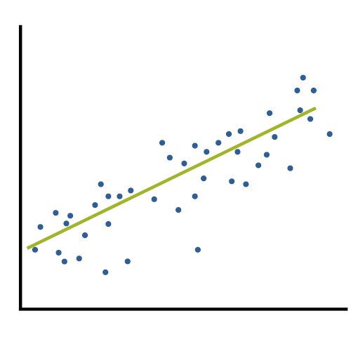
If you think about it, many familiar statistics fit this description. Regression coefficients give information about the magnitude and direction of the relationship between two variables. So do correlation coefficients. (more…)
One of the most difficult steps in calculating sample size estimates is determining the smallest scientifically meaningful effect size.
Here’s the logic:
The power of every significance test is based on four things: the alpha level, the size of the effect, the amount of variation in the data, and the sample size.
You will measure the effect size in question differently, depending on which statistical test you’re performing. It could be a mean difference, a difference in proportions, a correlation, regression slope, odds ratio, etc.
When you’re planning a study and estimating the sample size needed for (more…)
What is the difference between Clustered, Longitudinal, and Repeated Measures Data? You can use mixed models to analyze all of them. But the issues involved and some of the specifications you choose will differ.
Just recently, I came across a nice discussion about these differences in West, Welch, and Galecki’s (2007) excellent book, Linear Mixed Models.
It’s a common question. There is a lot of overlap in both the study design and in how you analyze the data from these designs.
West et al give a very nice summary of the three types. Here’s a paraphrasing of the differences as they explain them:
- In clustered data, the dependent variable is measured once for each subject, but the subjects themselves are somehow grouped (student grouped into classes, for example). There is no ordering to the subjects within the group, so their responses should be equally correlated.
- In repeated measures data, the dependent variable is measured more than once for each subject. Usually, there is some independent variable (often called a within-subject factor) that changes with each measurement.
- In longitudinal data, the dependent variable is measured at several time points for each subject, often over a relatively long period of time.
A Few Observations
West and colleagues also make the following good observations:
1. Dropout is usually not a problem in repeated measures studies, in which all data collection occurs in one sitting. It is a huge issue in longitudinal studies, which usually require multiple contacts with participants for data collection.
2. Longitudinal data can also be clustered. If you follow those students for two years, you have both clustered and longitudinal data. You have to deal with both.
3. It can be hard to distinguish between repeated measures and longitudinal data if the repeated measures occur over time. [My two cents: A pre/post/followup design is a classic example].
4. From an analysis point of view, it doesn’t really matter which one you have. All three are types of hierarchical, nested, or multilevel data. You would analyze them all with some sort of mixed or multilevel analysis. You may of course have extra issues (like dropout) to deal with in some of these.
My Own Observations
I agree with their observations, and I’d like to add a few from my own experience.
1. Repeated measures don’t have to be repeated over time. They can be repeated over space (the right knee gets the control operation and the left knee gets the experimental operation). They can also be repeated over condition (each subject gets both the high and low cognitive load condition. Longitudinal studies are pretty much always over time.
This becomes an issue mainly when you are choosing a covariance structure for the within-subject residuals (as determined by the Repeated statement in SAS’s Proc Mixed or SPSS Mixed). An auto-regressive structure is often needed when some repeated measurements are closer to each other than others (over either time or space). This is not an issue with purely clustered data, since there is no order to the observations within a cluster.
2. Time itself is often an important independent variable in longitudinal studies, but in repeated measures studies, it is usually confounded with some independent variable.
When you’re deciding on an analysis, it’s important to think about the role of time. Time is not important in an experiment, where each measurement is a different condition (with order often randomized). But it’s very important in a study designed to measure changes in a dependent variable over the course of 3 decades.
3. Time may be measured with some proxy like Age or Order. But it’s still really about time.
4. A longitudinal study does not have to be over years. You could be measuring reaction time every second for a minute. In cases like this, dropout isn’t an issue, although time is an important predictor.
5. Consider whether it makes sense to think about time as continuous or categorical. If you have only two time points, even if you have numerical measurements for them, there is no point in treating it as continuous. You need at least three time points to fit a line, but more is always better.
6. Longitudinal data can be analyzed with many statistical methods, including structural equation modeling and survival analysis. You only use multilevel modeling if the dependent variable is measured repeatedly and if the point of the model is to see how it changes (or differs).
Naming a data structure, design, or analysis is most helpful if it is so specific that it defines yours exactly. Your repeated measures analysis may not be like the repeated measures example you’re trying to follow. Rather than trying to name the analysis or the data structure, think about the issues involved in your design, your hypotheses, and your data. Work with them accordingly.
Go to the next article or see the full series on Easy-to-Confuse Statistical Concepts
If you’ve ever run a one-way analysis of variance (ANOVA), you’re familiar with post-hoc tests. The ANOVA omnibus test only tells you whether any groups differ in their means. But if you want to explore which specific group mean is different from which, you need to follow up with a post-hoc test. (more…)
One big advantage of R is its breadth. If anything has been done in statistics, there is an R package that will do it.
The problem is that sometimes there are four packages that will do it. This is big problem with R (and with Python for that matter). (more…)
When you need to compare a numeric outcome for two groups, what analysis do you think of first? Chances are, it’s the independent samples t-test. But that’s not the only, or always, the best option. In many situations, the Mann-Whitney U test is a better option.
The non-parametric Mann-Whitney U test is also called the Mann-Whitney-Wilcoxon test, or the Wilcoxon rank sum test. Non-parametric means that the hypothesis it’s testing is not about the parameter of a particular distribution.
It is part of a subgroup of non-parametric tests that are rank based. That means that the specific values of the outcomes are not important, only their order. In other words, we will be ranking the outcomes.
Like the t-test, this analysis tests whether two independent groups have similar typical outcomes. You can use it with numeric data, but unlike the t-test, it also works with ordinal data. Like the t-test, it is designed for comparisons, and not for estimation or prediction.
The biggest difference from the t-test is that it does not compare means. The Mann-Whitney U test determines whether a random observation from one group tends to be higher (or lower) than a random observation from the other group. Imagine choosing two observations, one from each group, over and over again. This test will determine whether one group is more likely to have the higher values.
It has many advantages: It is a straightforward comparison of means. There are versions for similar and different variances in the two groups. Many people are familiar with it.
(more…)
 When many of us hear “Effect Size Statistic,” we immediately think we need one of a few statistics: Eta-squared, Cohen’s d, R-squared.