 Centering variables is common practice in some areas, and rarely seen in others. That being the case, it isn’t always clear what are the reasons for centering variables.
 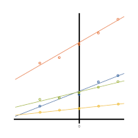 Is it only a matter of preference, or does centering variables help with analysis and interpretation? (more…)
Linear Regression
Member Training: Centering
November 30th, 2022 by TAF Support
Member Training: Analyzing Likert Scale Data
August 31st, 2022 by TAF Support
 Is it really ok to treat Likert items as continuous?
 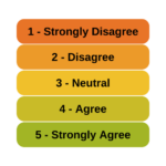 And can you just decide to combine Likert items to make a scale? Likert-type data is extremely common—and so are questions like these about how to analyze it appropriately. (more…)
The Difference Between R-squared and Adjusted R-squared
August 22nd, 2022 by Karen Grace-Martin
When is it important to use adjusted R-squared instead of R-squared?
R², the Coefficient of Determination, is one of the most useful and intuitive statistics we have in linear regression.
It tells you how well the model predicts the outcome and has some nice properties. But it also has one big drawback.
Member Training: Assumptions of Linear Models
June 30th, 2022 by TAF Support
What are the assumptions of linear models? If you compare two lists of assumptions, most of the time they’re not the same.
(more…)
When Linear Models Don’t Fit Your Data, Now What?
June 20th, 2022 by Karen Grace-Martin
When your dependent variable is not continuous, unbounded, and measured on an interval or ratio scale, linear models don’t fit. The data just will not meet the assumptions of linear models. But there’s good news, other models exist for many types of dependent variables.
Today I’m going to go into more detail about 6 common types of dependent variables that are either discrete, bounded, or measured on a nominal or ordinal scale and the tests that work for them instead. Some are all of these.
Linear Regression Analysis – 3 Common Causes of Multicollinearity and What Do to About Them
February 11th, 2022 by Karen Grace-Martin
Multicollinearity in regression is one of those issues that strikes fear into the hearts of researchers. You’ve heard about its dangers in statistics classes, and colleagues and journal reviews question your results because of it. But there are really only a few causes of multicollinearity. Let’s explore them.Multicollinearity is simply redundancy in the information contained in predictor variables. If the redundancy is moderate, (more…)
classes, and colleagues and journal reviews question your results because of it. But there are really only a few causes of multicollinearity. Let’s explore them.Multicollinearity is simply redundancy in the information contained in predictor variables. If the redundancy is moderate, (more…)