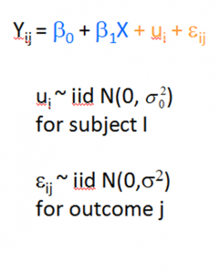
If you have run mixed models much at all, you have undoubtedly been haunted by some version of this very obtuse warning: “The  Hessian (or G or D) Matrix is not positive definite. Convergence has stopped.”
Or “The Model has not Converged. Parameter Estimates from the last iteration are displayed.”
What on earth does that mean?
Let’s start with some background. If you’ve never taken matrix algebra, (more…)
One issue in data analysis that feels like it should be obvious, but often isn’t, is setting up your data.
The kinds of issues involved include:
- What is a variable?

- What is a unit of observation?
- Which data should go in each row of the data matrix?
Answering these practical questions is one of those skills that comes with experience, especially in complicated data sets.
Even so, it’s extremely important. If the data isn’t set up right, the software won’t be able to run any of your analyses.
And in many data situations, you will need to set up the data different ways for different parts of the analyses. (more…)
Imputation as an approach to missing data has been around for decades.

You probably learned about mean imputation in methods classes, only to be told to never do it for a variety of very good reasons. Mean imputation, in which each missing value is replaced, or imputed, with the mean of observed values of that variable, is not the only type of imputation, however. (more…)
Updated 8/18/2021
I recently was asked whether to report means from descriptive statistics or from the Estimated Marginal Means with SPSS GLM.
The short answer: Report the Estimated Marginal Means (almost always).
To understand why and the rare case it doesn’t matter, let’s dig in a bit with a longer answer.
First, a marginal mean is the mean response for each category of a factor, adjusted for any other variables in the model (more on this later).
Just about any time you include a factor in a linear model, you’ll want to report the mean for each group. The F test of the model in the ANOVA table will give you a p-value for the null hypothesis that those means are equal. And that’s important.
But you need to see the means and their standard errors to interpret the results. The difference in those means is what measures the effect of the factor. While that difference can also appear in the regression coefficients, looking at the means themselves give you a context and makes interpretation more straightforward. This is especially true if you have interactions in the model.
Some basic info about marginal means
- In SPSS menus, they are in the Options button and in SPSS’s syntax they’re EMMEANS.
- These are called LSMeans in SAS, margins in Stata, and emmeans in R’s emmeans package.
- Although I’m talking about them in the context of linear models, all the software has them in other types of models, including linear mixed models, generalized linear models, and generalized linear mixed models.
- They are also called predicted means, and model-based means. There are probably a few other names for them, because that’s what happens in statistics.
When marginal means are the same as observed means
Let’s consider a few different models. In all of these, our factor of interest, X, is a categorical predictor for which we’re calculating Estimated Marginal Means. We’ll call it the Independent Variable (IV).
Model 1: No other predictors
If you have just a single factor in the model (a one-way anova), marginal means and observed means will be the same.
Observed means are what you would get if you simply calculated the mean of Y for each group of X.
Model 2: Other categorical predictors, and all are balanced
Likewise, if you have other factors in the model, if all those factors are balanced, the estimated marginal means will be the same as the observed means you got from descriptive statistics.
Model 3: Other categorical predictors, unbalanced
Now things change. The marginal mean for our IV is different from the observed mean. It’s the mean for each group of the IV, averaged across the groups for the other factor.
When you’re observing the category an individual is in, you will pretty much never get balanced data. Even when you’re doing random assignment, balanced groups can be hard to achieve.
In this situation, the observed means will be different than the marginal means. So report the marginal means. They better reflect the main effect of your IV—the effect of that IV, averaged across the groups of the other factor.
Model 4: A continuous covariate
When you have a covariate in the model the estimated marginal means will be adjusted for the covariate. Again, they’ll differ from observed means.
It works a little bit differently than it does with a factor. For a covariate, the estimated marginal mean is the mean of Y for each group of the IV at one specific value of the covariate.
By default in most software, this one specific value is the mean of the covariate. Therefore, you interpret the estimated marginal means of your IV as the mean of each group at the mean of the covariate.
This, of course, is the reason for including the covariate in the model–you want to see if your factor still has an effect, beyond the effect of the covariate. You are interested in the adjusted effects in both the overall F-test and in the means.
If you just use observed means and there was any association between the covariate and your IV, some of that mean difference would be driven by the covariate.
For example, say your IV is the type of math curriculum taught to first graders. There are two types. And say your covariate is child’s age, which is related to the outcome: math score.
It turns out that curriculum A has slightly older kids and a higher mean math score than curriculum B. Observed means for each curriculum will not account for the fact that the kids who received that curriculum were a little older. Marginal means will give you the mean math score for each group at the same age. In essence, it sets Age at a constant value before calculating the mean for each curriculum. This gives you a fairer comparison between the two curricula.
But there is another advantage here. Although the default value of the covariate is its mean, you can change this default. This is especially helpful for interpreting interactions, where you can see the means for each group of the IV at both high and low values of the covariate.
In SPSS, you can change this default using syntax, but not through the menus.
For example, in this syntax, the EMMEANS statement reports the marginal means of Y at each level of the categorical variable X at the mean of the Covariate V.
UNIANOVA Y BY X WITH V
/INTERCEPT=INCLUDE
/EMMEANS=TABLES(X) WITH(V=MEAN)
/DESIGN=X V.
If instead, you wanted to evaluate the effect of X at a specific value of V, say 50, you can just change the EMMEANS statement to:
/EMMEANS=TABLES(X) WITH(V=50)
Another good reason to use syntax.
Of all the stressors you’ve got right now, accessing your statistical software from home shouldn’t be one of them. (You know, the one on your office computer).
We’ve gotten some updates from some statistical software companies on how they’re making it easier to access the software you have a license to or to extend a free trial while you’re working from home.
(more…)
Learning how to analyze data can be frustrating at times. Why do statistical software companies have to add to our confusion?
I do not have a good answer to that question. What I will do is show examples. In upcoming blog posts, I will explain what each output means and how they are used in a model.
We will focus on ANOVA and linear regression models using SPSS and Stata software. As you will see, the biggest differences are not across software, but across procedures in the same software.
(more…)
 Hessian (or G or D) Matrix is not positive definite. Convergence has stopped.”


