One issue that affects how to interpret regression coefficients is the scale of the variables. In linear regression, the scaling of both the response variable Y, and the relevant predictor X, are both important.
In regression models like logistic regression, where the response variable is categorical, and therefore doesn’t have a numerical scale, this only applies to predictor variables, X.
This can be an issue of measurement units–miles vs. kilometers. Or it can be an issue of simply how big “one unit” is. For example, whether one unit of annual income is measured in dollars, thousands of dollars, or millions of dollars.
The good news is you can easily change the scale of variables to make it easier to interpret their regression coefficients. This works as well for functions of regression coefficients, like odds ratios and rate ratios.
All you have to do is create a new variable in your data set (don’t overwrite the individual one in case you make a mistake). This new variable is simply the old one multiplied or divided by some constant. The constant is often a factor of 10, but it doesn’t have to be. Then use the new variable in your model instead of the original one.
Since regression coefficients and odds ratios tell you the effect of a one unit change in the predictor, you should multiply them so that a one unit change in the predictor makes sense.
An Example of Rescaling Predictors
Here is a really simple example that I use in one of my workshops.
Y= first semester college GPA
X1= high school GPA
X2=SAT score
High School and first semester College GPA are both measured on a scale from 0 to 4. If you’re not familiar with this scaling, a 0 means you failed a class. An A (usually the top possible score) is a 4, a B is a 3, a C is a 2, and a D is a 1. So for a grade point average, a one point difference is very big.
If you’re an admissions counselor looking at high school transcripts, there is a big difference between a 3.7 GPA and a 2.7 GPA.
SAT score is on an entirely different scale. It’s a normed scale, so that the minimum is 200, the maximum is 800, and the mean is 500. Scores are in units of 10. You literally cannot receive a score of 622. You can get only 620 or 630.
So a one-point difference is not only tiny, it’s meaningless. Even a 10 point difference in SAT scores is pretty small. But 50 points is meaningful, and 100 points is large.
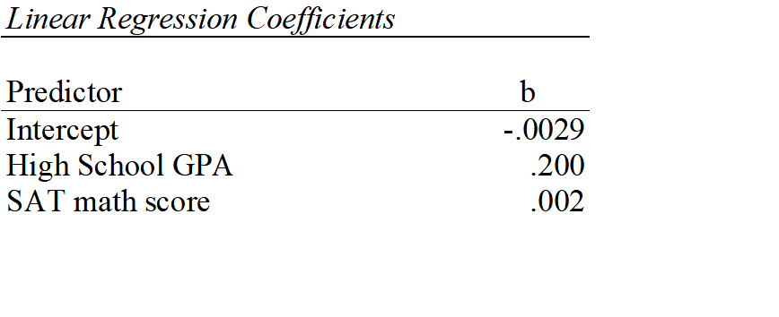
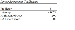
If you leave both predictors on the original scale in a regression that predicts first semester GPA, you get the following results:
 Let’s interpret those coefficients.
The coefficient for high school GPA here is .20. This says that for each one-unit difference in GPA, we expect, on average, a .2 higher first semester GPA. While a one-unit change in GPA is huge, that’s reasonably meaningful.
The coefficient for SAT math scores is .002. That looks tiny. It says that for each one-unit difference in SAT math score, we expect, on average, a .002 higher first semester GPA. But a one-unit difference in SAT score is too small to interpret. It’s too small to be meaningful.
So we can change the scaling of our SAT score predictor to be in 10-point differences. Or in 100 point differences. Chose the scale for which one unit is meaningful.
Changing the scale by mulitplying the coefficient
In a linear model, you can simply multiply the coefficient by 10 to reflect a 10-point difference. That’s a coefficient of .02. So for each 10 point difference in math SAT score we expect, on average, a .02 higher first semester GPA.
Or we could multiply the coefficient by 50 to reflect a 50-point difference. That’s a coefficient of .10. So for each 50 point difference in math SAT score we expect, on average, a .1 higher first semester GPA.
When it’s easier to just change the variables
Multiplying the coefficient is easier than rescaling the original variable if you only have one or two of these and you’re using linear regression.
It doesn’t work once you’ve done any sort of back-transformation in generalized linear models. So you can’t just multiply the odds ratio or the incidence rate ratio by 10 or 50. Both of these are created by exponentiating the regression coefficient. Because of the order of operations in algebra, You have to first multiply the coefficient by the constant, and then re-expontiate.
Likewise, if you are using this predictor in more than one linear regression model, it’s much simpler to rescale the variable in the first place. Simply divide that SAT score by 10 or 50 and the coefficient will .02 or .10, respectively.
Updated 12/2/2021
 classes, and colleagues and journal reviews question your results because of it. But there are really only a few causes of multicollinearity. Let’s explore them.Multicollinearity is simply redundancy in the information contained in predictor variables. If the redundancy is moderate, (more…)