In our last post, we calculated Pearson and Spearman correlation coefficients in R and got a surprising result.
So let’s investigate the data a little more with a scatter plot.
We use the same version of the data set of tourists. We have data on tourists from different nations, their gender, number of children, and how much they spent on their trip.
Again we copy and paste the following array into R.
M <- structure(list(COUNTRY = structure(c(3L, 3L, 3L, 3L, 1L, 3L, 2L, 3L, 1L, 3L, 3L, 1L, 2L, 2L, 3L, 3L, 3L, 2L, 3L, 1L, 1L, 3L,

1L, 2L), .Label = c("AUS", "JAPAN", "USA"), class = "factor"),GENDER = structure(c(2L, 1L, 2L, 2L, 1L, 2L, 1L, 2L, 1L, 2L, 2L, 1L, 1L, 1L, 1L, 2L, 1L, 1L, 2L, 2L, 1L, 1L, 1L, 2L), .Label = c("F", "M"), class = "factor"), CHILDREN = c(2L, 1L, 3L, 2L, 2L, 3L, 1L, 0L, 1L, 0L, 1L, 2L, 2L, 1L, 1L, 1L, 0L, 2L, 1L, 2L, 4L, 2L, 5L, 1L), SPEND = c(8500L, 23000L, 4000L, 9800L, 2200L, 4800L, 12300L, 8000L, 7100L, 10000L, 7800L, 7100L, 7900L, 7000L, 14200L, 11000L, 7900L, 2300L, 7000L, 8800L, 7500L, 15300L, 8000L, 7900L)), .Names = c("COUNTRY", "GENDER", "CHILDREN", "SPEND"), class = "data.frame", row.names = c(NA, -24L))
 M

attach(M)
plot(CHILDREN, SPEND)
(more…)
Let’s use R to explore bivariate relationships among variables.
Part 7 of this series showed how to do a nice bivariate plot, but it’s also useful to have a correlation statistic.
We use a new version of the data set we used in Part 20 of tourists from different nations, their gender, and number of children. Here, we have a new variable – the amount of money they spend while on vacation.
First, if the data object (A) for the previous version of the tourists data set is present in your R workspace, it is a good idea to remove it because it has some of the same variable names as the data set that you are about to read in. We remove A as follows:
rm(A)
Removing the object A ensures no confusion between different data objects that contain variables with similar names.
Now copy and paste the following array into R.
M <- structure(list(COUNTRY = structure(c(3L, 3L, 3L, 3L, 1L, 3L, 2L, 3L, 1L, 3L, 3L, 1L, 2L, 2L, 3L, 3L, 3L, 2L, 3L, 1L, 1L, 3L,

1L, 2L), .Label = c("AUS", "JAPAN", "USA"), class = "factor"),GENDER = structure(c(2L, 1L, 2L, 2L, 1L, 2L, 1L, 2L, 1L, 2L, 2L, 1L, 1L, 1L, 1L, 2L, 1L, 1L, 2L, 2L, 1L, 1L, 1L, 2L), .Label = c("F", "M"), class = "factor"), CHILDREN = c(2L, 1L, 3L, 2L, 2L, 3L, 1L, 0L, 1L, 0L, 1L, 2L, 2L, 1L, 1L, 1L, 0L, 2L, 1L, 2L, 4L, 2L, 5L, 1L), SPEND = c(8500L, 23000L, 4000L, 9800L, 2200L, 4800L, 12300L, 8000L, 7100L, 10000L, 7800L, 7100L, 7900L, 7000L, 14200L, 11000L, 7900L, 2300L, 7000L, 8800L, 7500L, 15300L, 8000L, 7900L)), .Names = c("COUNTRY", "GENDER", "CHILDREN", "SPEND"), class = "data.frame", row.names = c(NA, -24L))
 M

attach(M)
Do tourists with greater numbers of children spend more? Let’s calculate the correlation between CHILDREN and SPEND, using the cor() function.
R <- cor(CHILDREN, SPEND)

[1] -0.2612796
We have a weak correlation, but it’s negative! Tourists with a greater number of children tend to spend less rather than more!
(Even so, we’ll plot this in our next post to explore this unexpected finding).
We can round to any number of decimal places using the round() command.
round(R, 2)

[1] -0.26
The percentage of shared variance (100*r2) is:
100 * (R**2)

[1] 6.826704
To test whether your correlation coefficient differs from 0, use the cor.test() command.
cor.test(CHILDREN, SPEND)

 Pearson's product-moment correlation

data: CHILDREN and SPEND

t = -1.2696, df = 22, p-value = 0.2175

alternative hypothesis: true correlation is not equal to 0

95 percent confidence interval:

-0.6012997 0.1588609

sample estimates:

cor

-0.2612796
The cor.test() command returns the correlation coefficient, but also gives the p-value for the correlation. In this case, we see that the correlation is not significantly different from 0 (p is approximately 0.22).
Of course we have only a few values of the variable CHILDREN, and this fact will influence the correlation. Just how many values of CHILDREN do we have? Can we use the levels() command directly? (Recall that the term “level” has a few meanings in statistics, once of which is the values of a categorical variable, aka “factor“).
levels(CHILDREN)

NULL
R does not recognize CHILDREN as a factor. In order to use the levels() command, we must turn CHILDREN into a factor temporarily, using as.factor().
levels(as.factor(CHILDREN))

[1] "0" "1" "2" "3" "4" "5"
So we have six levels of CHILDREN. CHILDREN is a discrete variable without many values, so a Spearman correlation can be a better option. Let’s see how to implement a Spearman correlation:
cor(CHILDREN, SPEND, method ="spearman")

[1] -0.3116905
We have obtained a similar but slightly different correlation coefficient estimate because the Spearman correlation is indeed calculated differently than the Pearson.
Why not plot the data? We will do so in our next post.
About the Author: David Lillis has taught R to many researchers and statisticians. His company, Sigma Statistics and Research Limited, provides both on-line instruction and face-to-face workshops on R, and coding services in R. David holds a doctorate in applied statistics.
See our full R Tutorial Series and other blog posts regarding R programming.
Sometimes when you’re learning a new stat software package, the most frustrating part is not knowing how to do very basic things. This is especially frustrating if you already know how to do them in some other software.
Let’s look at some basic but very useful commands that are available in R.
We will use the following data set of tourists from different nations, their gender and numbers of children. Copy and paste the following array into R.
A <- structure(list(NATION = structure(c(3L, 3L, 3L, 1L, 3L, 2L, 3L,
1L, 3L, 3L, 1L, 2L, 2L, 3L, 3L, 3L, 2L), .Label = c("CHINA",
"GERMANY", "FRANCE"), class = "factor"), GENDER = structure(c(1L,
2L, 2L, 1L, 2L, 1L, 2L, 1L, 2L, 2L, 1L, 1L, 1L, 1L, 2L, 1L, 1L
), .Label = c("F", "M"), class = "factor"), CHILDREN = c(1L,
3L, 2L, 2L, 3L, 1L, 0L, 1L, 0L, 1L, 2L, 2L, 1L, 1L, 1L, 0L, 2L
)), .Names = c("NATION", "GENDER", "CHILDREN"), row.names = 2:18, class = "data.frame")
Want to check that R read the variables correctly? We can look at the first 3 rows using the head() command, as follows:
head(A, 3)
  NATION   GENDER   CHILDREN
2 FRANCE      F        1
3 FRANCE      M        3
4 FRANCE      M        2
Now we look at the last 4 rows using the tail() command:
tail(A, 4)
    NATION   GENDER  CHILDREN
15  FRANCE      F        1
16  FRANCE      M        1
17  FRANCE      F        0
18 GERMANY      F        2
Now we find the number of rows and number of columns using nrow() and ncol().
nrow(A)
[1] 17

ncol(A)
[1] 3
So we have 17 rows (cases) and three columns (variables). These functions look very basic, but they turn out to be very useful if you want to write R-based software to analyse data sets of different dimensions.
Now let’s attach A and check for the existence of particular data.
attach(A)
As you may know, attaching a data object makes it possible to refer to any variable by name, without having to specify the data object which contains that variable.
Does the USA appear in the NATION variable? We use the any() command and put USA inside quotation marks.
any(NATION == "USA")
[1] FALSE
Clearly, we do not have any data pertaining to the USA.
What are the values of the variable NATION?
levels(NATION)
[1] "CHINA"   "GERMANY" "FRANCE"
How many non-missing observations do we have in the variable NATION?
length(NATION)
[1] 17
OK, but how many different values of NATION do we have?
length(levels(NATION))
[1] 3
We have three different values.
Do we have tourists with more than three children? We use the any() command to find out.
any(CHILDREN > 3)
[1] FALSE
None of the tourists in this data set have more than three children.
Do we have any missing data in this data set?
In R, missing data is indicated in the data set with NA.
any(is.na(A))
[1] FALSE
We have no missing data here.
Which observations involve FRANCE? We use the which() command to identify the relevant indices, counting column-wise.
which(A == "FRANCE")
[1]  1  2  3  5  7  9 10 14 15 16
How many observations involve FRANCE? We wrap the above syntax inside the length() command to perform this calculation.
length(which(A == "FRANCE"))
[1] 10
We have a total of ten such observations.
That wasn’t so hard! In our next post we will look at further analytic techniques in R.
About the Author: David Lillis has taught R to many researchers and statisticians. His company, Sigma Statistics and Research Limited, provides both on-line instruction and face-to-face workshops on R, and coding services in R. David holds a doctorate in applied statistics.
See our full R Tutorial Series and other blog posts regarding R programming.
I mentioned in my last post that R Commander can do a LOT of data manipulation, data analyses, and graphs in R without you ever having to program anything.
Here I want to give you some examples, so you can see how truly useful this is.
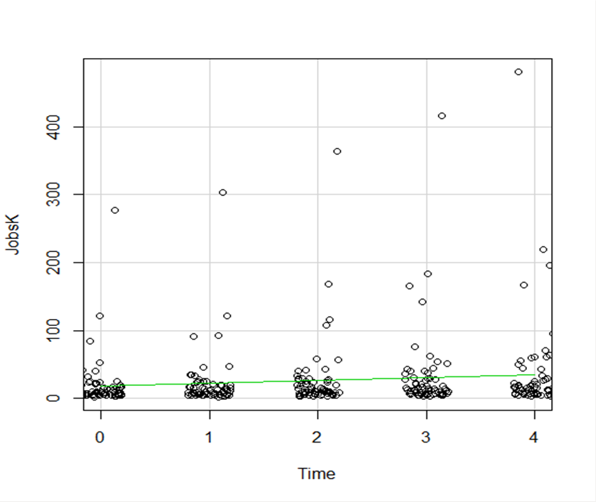
Let’s start with a simple scatter plot between Time and the number of Jobs (in thousands) in 67 counties. Time is measured in decades since 1960.
The green line is the best fit linear regression line.
This wasn’t the default in R Commander (I actually had to remove a few things to get to this), but it’s a useful way to start out.
A few ways we can easily customize this graph:
Jittering
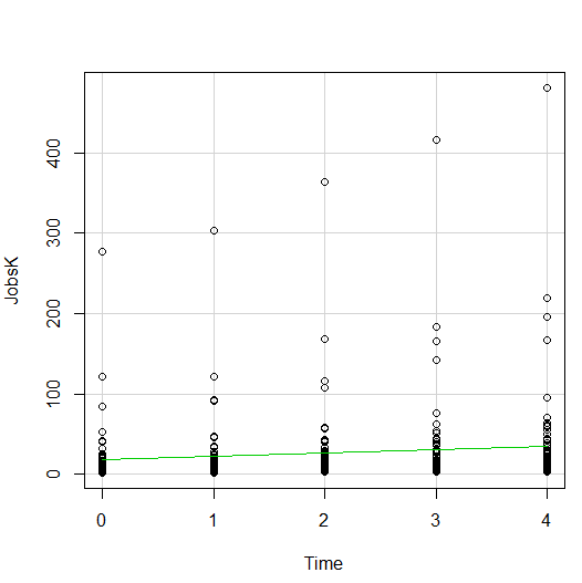
We see here a common issue in scatter plots–because the X values are discrete, the points are all on top of each other.
It’s difficult to tell just how many points there are at the bottom of the graph–it’s just a mass of black.
One great way to solve this is by jittering the points.
All this means is that instead of putting identical points right on top of each other, we move it slightly, randomly, in either one or both directions. In this example, I jittered only horizontally:
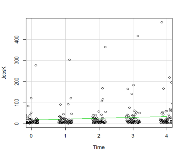
So while the points aren’t graphed exactly where they are, we can see the trends and we can now see how many points there are in each decade.
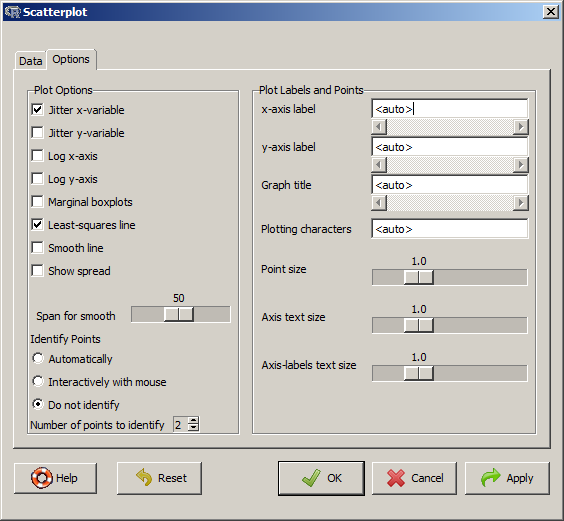
How hard is this to do in R Commander? One click:
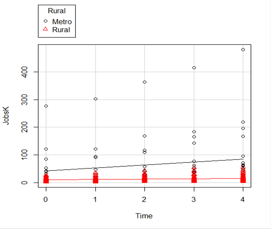
Regression Lines by Group
Another useful change to a scatter plot is to add a separate regression line to the graph based on some sort of factor in the data set.
In this example, the observations are measured for counties and each county is classified as being either Rural or Metropolitan.
If we’d like to see if the growth in jobs over time is different in Rural and Metropolitan counties, we need a separate line for each group.
In R Commander we can do this quite easily. Not only do we get two regression lines, but each point is clearly designated as being from either a Rural or Metropolitan county through its color and shape.
It’s quite clear that not only was there more growth in the number of jobs in Metro counties, there was almost no change at all in the Rural counties.
 And once again, how difficult is this? This time, two clicks.
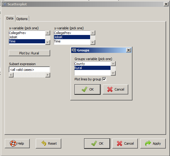
There are quite a few modifications you can make just using the buttons, but of course, R Commander doesn’t do everything.
For example, I could not figure out how to change those red triangles to green rectangles through the menus.
But that’s the best part about R Commander. It works very much like the Paste button in SPSS.
Meaning, it creates the code for you. So I can take the code it created, then edit it to get my graph looking the way I want.
I don’t have to memorize which command creates a scatter plot.
I don’t have to memorize how to pull my SPSS data into R or tell R that Rural is a factor. I can do all that through R Commander, then just look up the option to change the color and shape of the red triangles.
I received a question recently about R Commander, a free R package.
R Commander overlays a menu-based interface to R, so just like SPSS or JMP, you can run analyses using menus. Nice, huh?
The question was whether R Commander does everything R does, or just a small subset.
Unfortunately, R Commander can’t do everything R does. Not even close.
But it does a lot. More than just the basics.
So I thought I would show you some of the things R Commander can do entirely through menus–no programming required, just so you can see just how unbelievably useful it is.
Since R commander is a free R package, it can be installed easily through R! Just type install.packages("Rcmdr") in the command line the first time you use it, then type library("Rcmdr") each time you want to launch the menus.
Data Sets and Variables
Import data sets from other software:
- SPSS
- Stata
- Excel
- Minitab
- Text
- SAS Xport
Define Numerical Variables as categorical and label the values
Open the data sets that come with R packages
Merge Data Sets
Edit and show the data in a data spreadsheet
Personally, I think that if this was all R Commander did, it would be incredibly useful. These are the types of things I just cannot remember all the commands for, since I just don’t use R often enough.
Data Analysis
Yes, R Commander does many of the simple statistical tests you’d expect:
- Chi-square tests
- Paired and Independent Samples t-tests
- Tests of Proportions
- Common nonparametrics, like Friedman, Wilcoxon, and Kruskal-Wallis tests
- One-way ANOVA and simple linear regression
What is surprising though, is how many higher-level statistics and models it runs:
- Hierarchical and K-Means Cluster analysis (with 7 linkage methods and 4 options of distance measures)
- Principal Components and Factor Analysis
- Linear Regression (with model selection, influence statistics, and multicollinearity diagnostic options, among others)
- Logistic regression for binary, ordinal, and multinomial responses
- Generalized linear models, including Gamma and Poisson models
In other words–you can use R Commander to run in R most of the analyses that most researchers need.
Graphs
A sample of the types of graphs R Commander creates in R without you having to write any code:
- QQ Plots
- Scatter plots
- Histograms
- Box Plots
- Bar Charts
The nice part is that it does not only do simple versions of these plots. You can, for example, add regression lines to a scatter plot or run histograms by a grouping factor.
If you’re ready to get started practicing, click here to learn about making scatterplots in R commander, or click here to learn how to use R commander to sample from a uniform distribution.
In the last lesson, we saw how to use qplot to map symbol colour to a categorical variable. Now we see how to control symbol colours and create legend titles.
M <- structure(list(PATIENT = c("Mary","Dave","Simon","Steve","Sue","Frida","Magnus","Beth","Peter","Guy","Irina","Liz"),

GENDER = c("F","M","M","M","F","F","M","F","M","M","F","F"),

TREATMENT = c("A","B","C","A","A","B","A","C","A","C","B","C"),

AGE =c("Y","M","M","E","M","M","E","E","M","E","M","M"),

WEIGHT_1 = c(79.2,58.8,72.0,59.7,79.6,83.1,68.7,67.6,79.1,39.9,64.7,65.6),

WEIGHT_2 = c(76.6,59.3,70.1,57.3,79.8,82.3,66.8,67.4,76.8,41.4,65.3,63.2),

HEIGHT = c(169,161,175,149,179,177,175,170,177,138,170,165),

SMOKE = c("Y","Y","N","N","N","N","N","N","N","N","N","Y"),

EXERCISE = c(TRUE,FALSE,FALSE,FALSE,TRUE,FALSE,FALSE,TRUE,TRUE,FALSE,FALSE,TRUE),

RECOVER = c(1,0,1,1,1,0,1,1,1,1,0,1)),

.Names = c("PATIENT","GENDER","TREATMENT","AGE","WEIGHT_1","WEIGHT_2","HEIGHT","SMOKE","EXERCISE","RECOVER"),

class = "data.frame", row.names = 1:12)
M
    PATIENT GENDER TREATMENT AGE WEIGHT_1 WEIGHT_2 HEIGHT SMOKE EXERCISE RECOVER
1     Mary      F         A   Y     79.2     76.6    169     Y     TRUE       1
2     Dave      M         B   M     58.8     59.3    161     Y    FALSE       0
3    Simon      M         C   M     72.0     70.1    175     N    FALSE       1
4    Steve      M         A   E     59.7     57.3    149     N    FALSE       1
5      Sue      F         A   M     79.6     79.8    179     N     TRUE       1
6    Frida      F         B   M     83.1     82.3    177     N    FALSE       0
7   Magnus      M         A   E     68.7     66.8    175     N    FALSE       1
8     Beth      F         C   E     67.6     67.4    170     N     TRUE       1
9    Peter      M         A   M     79.1     76.8    177     N     TRUE       1
10     Guy      M         C   E     39.9     41.4    138     N    FALSE       1
11   Irina      F         B   M     64.7     65.3    170     N    FALSE       0
12     Liz      F         C   M     65.6     63.2    165     Y     TRUE       1
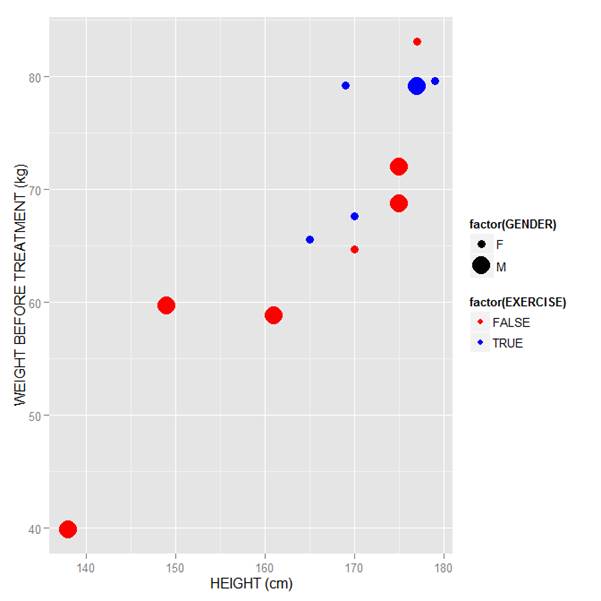
Now let’s map symbol size to GENDER and symbol colour to EXERCISE, but choosing our own colours. To control your symbol colours, use the layer: scale_colour_manual(values = c()) and select your desired colours. We choose red and blue, and symbol sizes 3 and 7.
qplot(HEIGHT, WEIGHT_1, data = M, geom = c("point"), xlab = "HEIGHT (cm)", ylab = "WEIGHT BEFORE TREATMENT (kg)" , size = factor(GENDER), color = factor(EXERCISE)) + scale_size_manual(values = c(3, 7)) + scale_colour_manual(values = c("red", "blue"))
Here is our graph with red and blue points:
Now let’s see how to control the legend title (the title that sits directly above the legend). For this example, we control the legend title through the name argument within the two functions scale_size_manual() and scale_colour_manual(). Enter this syntax in which we choose appropriate legend titles:
qplot(HEIGHT, WEIGHT_1, data = M, geom = c("point"), xlab = "HEIGHT (cm)", ylab = "WEIGHT BEFORE TREATMENT (kg)" , size = factor(GENDER), color = factor(EXERCISE)) + scale_size_manual(values = c(3, 7), name="Gender") + scale_colour_manual(values = c("red","blue"), name="Exercise")
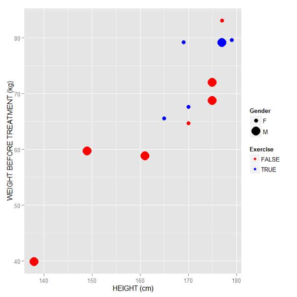
We now have our preferred symbol colour and size, and legend titles of our choosing.
That wasn’t so hard! In our next blog post we will learn about plotting regression lines in R.
About the Author: David Lillis Ph. D. has taught R to many researchers and statisticians. His company, Sigma Statistics and Research Limited, provides both on-line instruction and face-to-face workshops on R, and coding services in R. David holds a doctorate in applied statistics.
See our full R Tutorial Series and other blog posts regarding R programming.