
In Part 3 we used the lm() command to perform least squares regressions. In Part 4 we will look at more advanced aspects of regression models and see what R has to offer.
One way of checking for non-linearity in your data is to fit a polynomial model and check whether the polynomial model fits the data better than a linear model. However, you may also wish to fit a quadratic or higher model because you have reason to believe that the relationship between the variables is inherently polynomial in nature. Let’s see how to fit a quadratic model in R.
We will use a data set of counts of a variable that is decreasing over time. Cut and paste the following data into your R workspace.
A <- structure(list(Time = c(0, 1, 2, 4, 6, 8, 9, 10, 11, 12, 13,
14, 15, 16, 18, 19, 20, 21, 22, 24, 25, 26, 27, 28, 29, 30),
Counts = c(126.6, 101.8, 71.6, 101.6, 68.1, 62.9, 45.5, 41.9,
46.3, 34.1, 38.2, 41.7, 24.7, 41.5, 36.6, 19.6,
22.8, 29.6, 23.5, 15.3, 13.4, 26.8, 9.8, 18.8, 25.9, 19.3)), .Names = c("Time", "Counts"),
row.names = c(1L, 2L, 3L, 5L, 7L, 9L, 10L, 11L, 12L, 13L, 14L, 15L, 16L, 17L, 19L, 20L, 21L, 22L, 23L, 25L, 26L, 27L, 28L, 29L, 30L, 31L),
class = "data.frame")
Let’s attach the entire dataset so that we can refer to all variables directly by name.
attach(A)
names(A)
First, let’s set up a linear model, though really we should plot first and only then perform the regression.
linear.model <-lm(Counts ~ Time)
We now obtain detailed information on our regression through the summary() command.
summary(linear.model)
Call:
lm(formula = Counts ~ Time)

Residuals:
   Min     1Q Median     3Q     Max
-20.084 -9.875 -1.882   8.494 39.445

Coefficients:
           Estimate Std. Error t value Pr(>|t|)
(Intercept) 87.1550     6.0186 14.481 2.33e-13 ***
Time         -2.8247     0.3318 -8.513 1.03e-08 ***
---
Signif. codes: 0 ‘***’ 0.001 ‘**’ 0.01 ‘*’ 0.05 ‘.’ 0.1 ‘ ’ 1

Residual standard error: 15.16 on 24 degrees of freedom
Multiple R-squared: 0.7512,   Adjusted R-squared: 0.7408
F-statistic: 72.47 on 1 and 24 DF, p-value: 1.033e-08
The model explains over 74% of the variance and has highly significant coefficients for the intercept and the independent variable and also a highly significant overall model p-value. However, let’s plot the counts over time and superpose our linear model.
plot(Time, Counts, pch=16, ylab = "Counts ", cex.lab = 1.3, col = "red" )

abline(lm(Counts ~ Time), col = "blue")
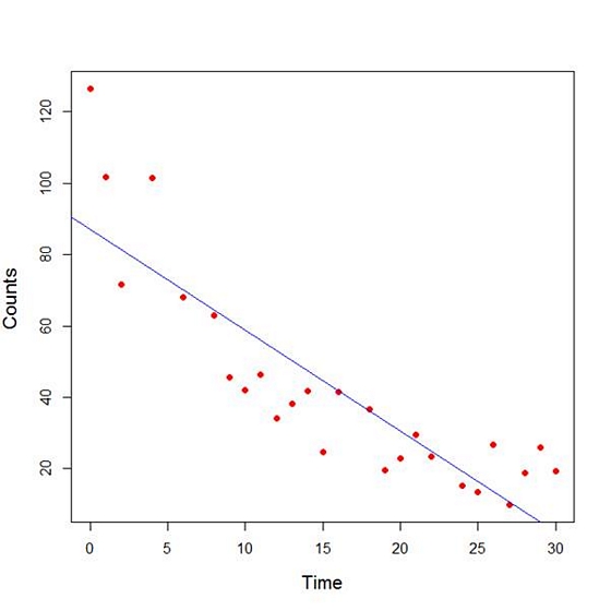
Here the syntax cex.lab = 1.3 produced axis labels of a nice size.
The model looks good, but we can see that the plot has curvature that is not explained well by a linear model. Now we fit a model that is quadratic in time. We create a variable called Time2 which is the square of the variable Time.
Time2 <- Time^2
quadratic.model <-lm(Counts ~ Time + Time2)
Note the syntax involved in fitting a linear model with two or more predictors. We include each predictor and put a plus sign between them.
summary(quadratic.model)
Call:
lm(formula = Counts ~ Time + Time2)
Residuals:
     Min       1Q   Median       3Q     Max
-24.2649 -4.9206 -0.9519   5.5860 18.7728

Coefficients:
             Estimate Std. Error t value Pr(>|t|)
(Intercept) 110.10749   5.48026 20.092 4.38e-16 ***
Time         -7.42253   0.80583 -9.211 3.52e-09 ***
Time2         0.15061   0.02545   5.917 4.95e-06 ***
---
Signif. codes: 0 ‘***’ 0.001 ‘**’ 0.01 ‘*’ 0.05 ‘.’ 0.1 ‘ ’ 1

Residual standard error: 9.754 on 23 degrees of freedom
Multiple R-squared: 0.9014,   Adjusted R-squared: 0.8928
F-statistic: 105.1 on 2 and 23 DF, p-value: 2.701e-12
Our quadratic model is essentially a linear model in two variables, one of which is the square of the other. We see that however good the linear model was, a quadratic model performs even better, explaining an additional 15% of the variance. Now let’s plot the quadratic model by setting up a grid of time values running from 0 to 30 seconds in increments of 0.1s.
timevalues <- seq(0, 30, 0.1)
predictedcounts <- predict(quadratic.model,list(Time=timevalues, Time2=timevalues^2))
plot(Time, Counts, pch=16, xlab = "Time (s)", ylab = "Counts", cex.lab = 1.3, col = "blue")
Now we include the quadratic model to the plot using the lines() command.
lines(timevalues, predictedcounts, col = "darkgreen", lwd = 3)
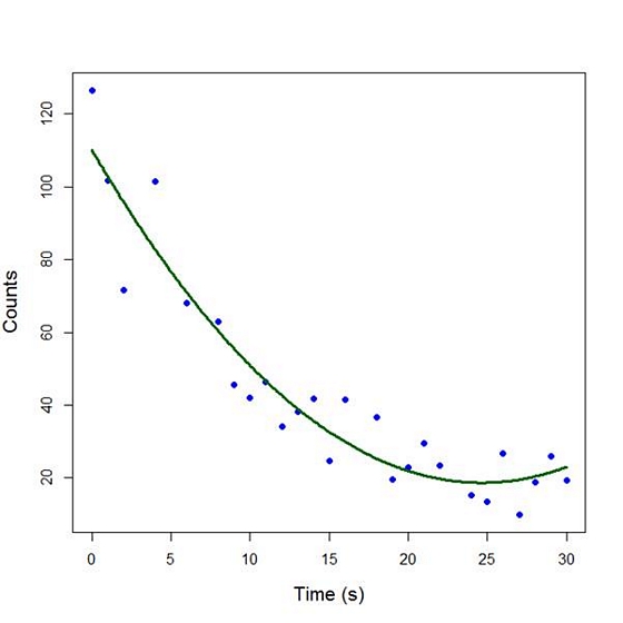
The quadratic model appears to fit the data better than the linear model. We will look again at fitting curved models in our next blog post.
About the Author: David Lillis has taught R to many researchers and statisticians. His company, Sigma Statistics and Research Limited, provides both on-line instruction and face-to-face workshops on R, and coding services in R. David holds a doctorate in applied statistics.
See our full R Tutorial Series and other blog posts regarding R programming.
One of the nice features of SPSS is its ability to keep track of information on the variables themselves.

This includes variable labels, missing data codes, value labels, and variable formats. Spending the time to set up variable information makes data analysis much easier–you don’t have to keep looking up whether males are coded 1 or 0, for example.
And having them all in the variable view window makes things incredibly easy while you’re doing your analysis. But sometimes you need to just print them all out–to create a code book for another analyst or to include in the output you’re sending to a collaborator. Or even just to print them out for yourself for easy reference.
There is a nice little way to get a few tables with a list of all the variable metadata. It’s in the File menu. Simply choose Display Data File Information and Working File.
Doing this gives you two tables. The first includes the following information on the variables. I find the information I use the most are the labels and the missing data codes.


Even more useful, though, is the Value Label table.
It lists out the labels for all the values for each variable.
So you don’t have to remember that Job Category (jobcat) 1 is “Clerical,” 2 is “Custodial,” and 3 is “Managerial.”
It’s all right there.
by Maike Rahn, PhD
In the previous blogs I wrote about the basics of running a factor analysis. Real-life factor analysis can become complicated. Here are some of the more common problems researchers encounter and some possible solutions:
- The factor loadings in your confirmatory factor analysis are only |0.5| or less.
Solution: lower the cut-offs of your factor loadings, provided that lower factor loadings are expected and accepted in your field.
- Your confirmatory factor analysis does not show the hypothesized number of factors.
Solution 1: you were not able to validate the factor structure in your sample; your analysis with this sample did not work out.
Solution 2: your factor analysis has just become exploratory. Something is going on with your sample that is different from the samples used in other studies. Find out what it is.
- A few key variables in your confirmatory factor analysis do not behave as expected and/or are correlated with the wrong factor.
Solution: the good news is that you found the hypothesized factors. The bad news is (more…)
Recently I gave a webinar The Steps to Running Any Statistical Model. A few hundred people were live on the webinar. We held a Q&A session at the end, but as you can imagine, we didn’t have time to get through all the questions.
This is the first in a series of written answers to some of those questions. I’ve tried to sort them by the step each is about.
A written list of the steps is available here.
If you missed the webinar, you can view the video here. It’s free.
Questions about Step 1. Write out research questions in theoretical and operational terms
Q: In using secondary data research designing, have you found that this type of data source affects the research question? That is, should one have a strong understanding of the data to ensure their theoretical concept can be operational to fit the data? My research question changes the more I learn.
Yes. There’s no point in asking research questions that the data you have available can’t answer.
So the order of the steps would have to change—you may have to start with a vague idea of the type of research question you want to ask, but only refine it after doing some descriptive statistics, or even running an initial model.
Q: How soon in the process should one start with the first group of steps?
You want to at least start thinking about them as you’re doing the lit review and formulating your research questions.
Think about how you could measure variables, which ones are likely to be collinear or have a lot of missing data. Think about the kind of model you’d have to do for each research question.
Think of a scenario where the same research question could be operationalized such that the dependent variable is measured either continuous or ordered categories. An easy example is income in dollars measured by actual income or by income categories.
By all means, if people can answer the question with a real and accurate number, your analysis will be much, much easier. In many situations, they can’t. They won’t know, remember, or tell you their exact income. If so, you may have to use categories to prevent missing data. But these are things to think about early.
Q: where in the process do you use existing lit/results to shape the research question and modeling?
I would start by putting the literature review before Step 1. You’ll use that to decide on a theoretical research question, as well as ways to operationalize it..
But it will help you other places as well. For example, it helps the sample size calculations to have variance estimates from other studies. Other studies may give you an idea of variables that are likely to have missing data, too little variation to include as predictors. They may change your exploratory factor analysis in Step 7 to a confirmatory one.
In fact, just about every step can benefit from a good literature review.
If you missed the webinar, you can view the video here. It’s free.