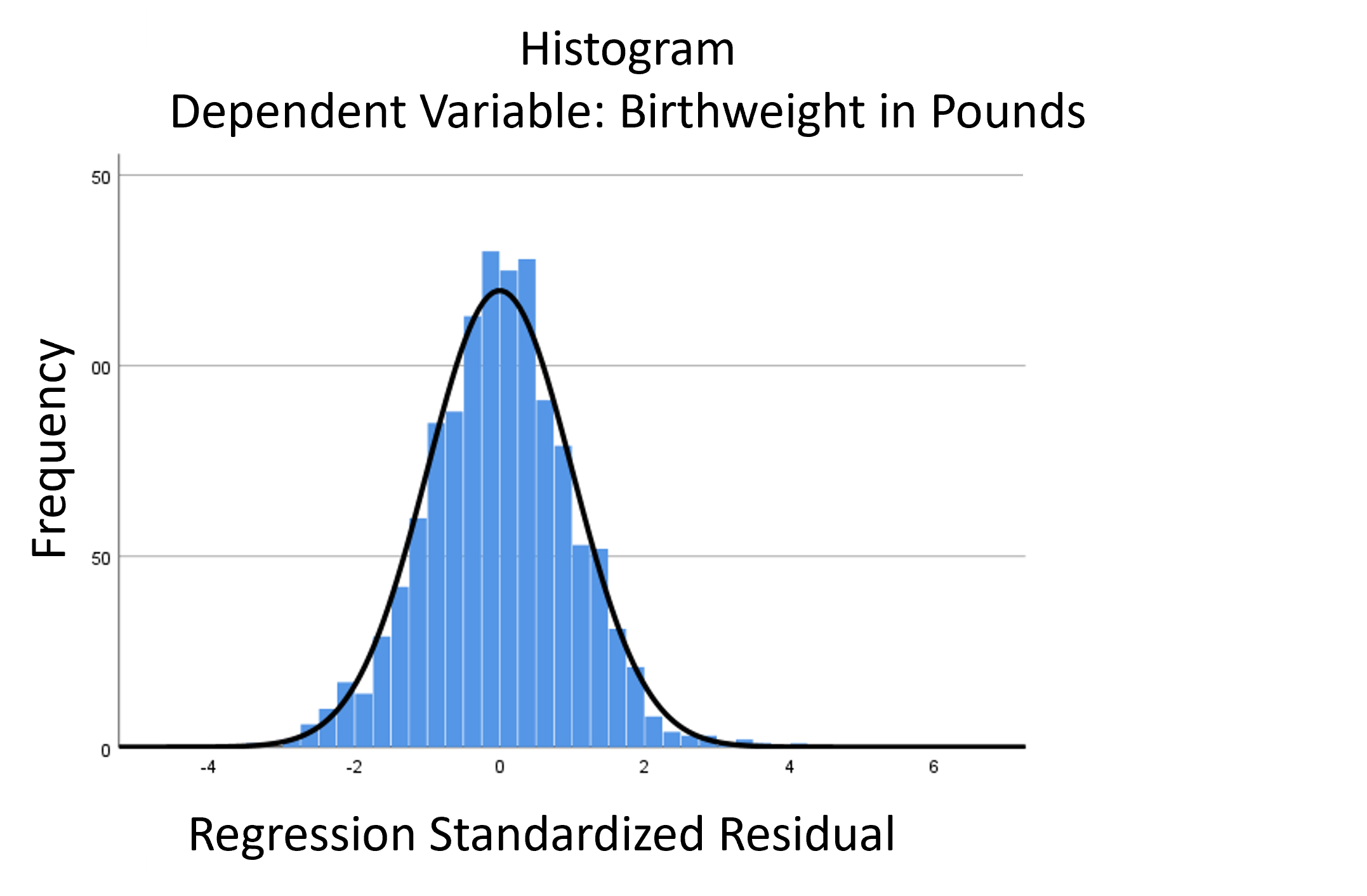
The linear model normality assumption, along with constant variance assumption, is quite robust to departures. That means that even if the 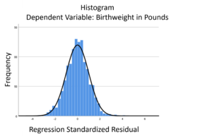 assumptions aren’t met perfectly, the resulting p-values and confidence intervals will still be reasonable estimates.
This is great because it gives you a bit of leeway to run linear models, which are intuitive and (relatively) straightforward. This is true for both linear regression and ANOVA.
You do need to check the assumptions anyway, though. You can’t just claim robustness and not check. Why? Because some departures are so far off that the p-values and confidence intervals become inaccurate. And in many cases there are remedial measures you can take to turn non-normal residuals into normal ones.
But sometimes you can’t.
Sometimes it’s because the dependent variable just isn’t appropriate for a linear model. The (more…)
Many variables we want to measure just can’t be directly measured with a single variable. Instead you have to combine a set of variables into a single index.
But how do you determine which variables to combine and how best to combine them?
Exploratory Factor Analysis.
EFA is a method for finding a measurement for one or more unmeasurable (latent) variables from a set of related observed variables. It is especially useful for scale construction.
In this webinar, you will learn through three examples an overview of EFA, including:
- The five steps to conducting an EFA
- Key concepts like rotation
- Factor scores
- The importance of interpretability
Note: This training is an exclusive benefit to members of the Statistically Speaking Membership Program and part of the Stat’s Amore Trainings Series. Each Stat’s Amore Training is approximately 90 minutes long.
About the Instructor

Karen Grace-Martin helps statistics practitioners gain an intuitive understanding of how statistics is applied to real data in research studies.
She has guided and trained researchers through their statistical analysis for over 15 years as a statistical consultant at Cornell University and through The Analysis Factor. She has master’s degrees in both applied statistics and social psychology and is an expert in SPSS and SAS.
Not a Member Yet?
It’s never too early to set yourself up for successful analysis with support and training from expert statisticians.
Just head over and sign up for Statistically Speaking.
You'll get access to this training webinar, 130+ other stats trainings, a pathway to work through the trainings that you need — plus the expert guidance you need to build statistical skill with live Q&A sessions and an ask-a-mentor forum.
SPSS has a nice little feature for adding and averaging variables with  missing data that many people don’t know about.
It allows you to add or average variables that have some missing data, while specifying how many are allowed to be missing. (more…)
You might be surprised to hear that not only can linear regression fit lines between a response variable Y and one or more predictor variables, X, it can fit curves too. There are many ways to do this, but the simplest is by adding a polynomial term.
So what is a polynomial term and how do you know you need one?
The linear parameters in a regression model
A linear regression model has a few key parameters. These include the intercept coefficient, the slope coefficient, and the residual variance.
That intercept defines the height of the regression line. It does so by measuring the height of the line at one specific point: when all X = 0.
The slope defines how much Y differs, on average, for each one unit difference in X. In other words, it measures the constant relationship between X and Y. Yes, there can be multiple Xs and each one has its own slope.
A polynomial term–a quadratic (squared) or cubic (cubed) term turns a linear regression model into a curve.
(more…)
No matter what statistical model you’re running, you need to take the same steps. The order and the specifics of  how you do each step will differ depending on the data and the type of model you use.
These steps are in 4 phases. Most people think of only the third as modeling. But the phases before this one are fundamental to making the modeling go well. It will be much, much easier, more accurate, and more efficient if you don’t skip them.
And there is no point in running the model if you skip the last phase. That’s where you communicate the results.
I’ve found that if I think of them all as part of the analysis, the modeling process is faster, easier, and makes more sense.
Phase 1: Define and Design
In the first five steps of running the model, the object is clarity. You want to make everything as clear as possible to yourself. The clearer things are at this point, the smoother everything will be. (more…)
 A well-fitting regression model results in predicted values close to the observed data values. The mean model, which uses the mean for every predicted value, generally would be used if there were no useful predictor variables. The fit of a proposed regression model should therefore be better than the fit of the mean model. But how do you measure that model fit?
(more…)
 assumptions aren’t met perfectly, the resulting p-values and confidence intervals will still be reasonable estimates.