new blog post: Member Training: The Dark Side of Data Science

Previous Posts
Pretty much all of the common statistical models we use, with the exception of OLS Linear Models, use Maximum Likelihood estimation. This includes favorites like: All Generalized Linear Models, including logistic, probit, Poisson, beta, negative binomial regression Linear Mixed Models Generalized Linear Mixed Models Parametric Survival Analysis models, like Weibull models Structural Equation Models That's a lot of models. If you've ever learned any of these, you've heard that some of the statistics that compare model fit in competing models require that models be nested. This is particularly important while you're trying to do model building.
Residuals can be a very broad topic - one that most everyone has heard of, but few people truly understand. It’s time to change that. By definition, a “residual” is “the quantity remaining after other things have been subtracted or allowed for.” In statistics, we use the term in a similar fashion. Residuals come in various forms: Standardized Studentized Pearson Deviance But which ones do we use… and why?
Often a model is not a simple process from a treatment or intervention to the outcome. In essence, the value of X does not always directly predict the value of Y. Mediators can affect the relationship between X and Y. Moderators can affect the scale and magnitude of that relationship. And sometimes the mediators and moderators affect each other.
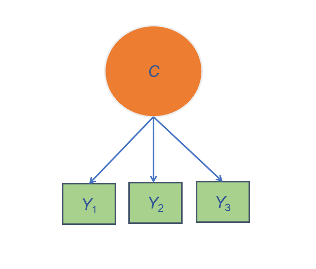
One of the most common—and one of the trickiest—challenges in data analysis is deciding how to include multiple predictors in a model, especially when they’re related to each other. Here's an example. Let's say you are interested in studying the relationship between work spillover into personal time as a predictor of job burnout. You have 5 categorical yes/no variables that indicate whether a particular symptom of work spillover is present (see below). While you could use each individual item, you're not really interested if one in particular is related to the outcome. Perhaps it's not really each symptom that's important, but the idea that spillover is happening. One possibility is to count up the number of items to which each respondent said yes. This variable will measure the degree to which spillover is happening. In many studies, this is just what you need. But it doesn't tell you something important—whether there are certain combinations that generally co-occur, and is it these combinations that affect burnout? In other words, what if it's not just the degree of spillover that's important, but the type? Enter Latent Class Analysis (LCA).
One question that seems to come up pretty often is: What is the difference between logistic and probit regression? Well, let’s start with how they’re the same: Both are types of generalized linear models. This means they have this form:
We often talk about nested factors in mixed models -- students nested in classes, observations nested within subject. But in all but the simplest designs, it's not that straightforward. In this webinar, you'll learn the difference between crossed and nested factors. We'll walk through a number of examples of different designs from real studies to pull apart which factors are crossed, which are nested, and which are somewhere in between. We'll also talk about a few classic designs, like split plots, Latin squares, and hierarchical data. Particular focus will be on how you can figure all this out in your own design and how it affects how you can and cannot analyze the data.
Linear regression with a continuous predictor is set up to measure the constant relationship between that predictor and a continuous outcome. This relationship is measured in the expected change in the outcome for each one-unit change in the predictor. One big assumption in this kind of model, though, is that this rate of change is the same for every value of the predictor. It's an assumption we need to question, though, because it's not a good approach for a lot of relationships. Segmented regression allows you to generate different slopes and/or intercepts for different segments of values of the continuous predictor. This can provide you with a wealth of information that a non-segmented regression cannot.
Here's a common situation. Your grant application or committee requires sample size estimates. It's not the calculations that are hard (though they can be), it's getting the information to fill into the calculations. Every article you read on it says you need to either use pilot data or another similar study as a basis for the values to enter into the software. You have neither. No similar studies have ever used the scale you're using for the dependent variable. And while you'd love to run a pilot study, it's just not possible. There are too many practical constraints -- time, money, distance, ethics. What do you do?
We’ve talked a lot around here about the reasons to use syntax — not only menus — in your statistical analyses. Regardless of which software you use, the syntax file is pretty much always a text file. This is true for R, SPSS, SAS, Stata — just about all of them. This is important because it means you can use an unlikely tool to help you code: Microsoft Word. I know what you're thinking. Word? Really? Yep, it's true. Essentially it's because Word has much better Search-and-Replace options than your stat software’s editor. Here are a couple features of Word’s search-and-replace that I use to help me code faster.
There are many rules of thumb in statistical analysis that make decision making and understanding results much easier. Have you ever stopped to wonder where these rules came from, let alone if there is any scientific basis for them? Is there logic behind these rules, or is it propagation of urban legends? In this webinar, we’ll explore and question the origins, justifications, and some of the most common rules of thumb in statistical analysis.
 stat skill-building compass