Updated 8/18/2021
I recently was asked whether to report means from descriptive statistics or from the Estimated Marginal Means with SPSS GLM.
The short answer: Report the Estimated Marginal Means (almost always).
To understand why and the rare case it doesn’t matter, let’s dig in a bit with a longer answer.
First, a marginal mean is the mean response for each category of a factor, adjusted for any other variables in the model (more on this later).
Just about any time you include a factor in a linear model, you’ll want to report the mean for each group. The F test of the model in the ANOVA table will give you a p-value for the null hypothesis that those means are equal. And that’s important.
But you need to see the means and their standard errors to interpret the results. The difference in those means is what measures the effect of the factor. While that difference can also appear in the regression coefficients, looking at the means themselves give you a context and makes interpretation more straightforward. This is especially true if you have interactions in the model.
Some basic info about marginal means
- In SPSS menus, they are in the Options button and in SPSS’s syntax they’re EMMEANS.
- These are called LSMeans in SAS, margins in Stata, and emmeans in R’s emmeans package.
- Although I’m talking about them in the context of linear models, all the software has them in other types of models, including linear mixed models, generalized linear models, and generalized linear mixed models.
- They are also called predicted means, and model-based means. There are probably a few other names for them, because that’s what happens in statistics.
When marginal means are the same as observed means
Let’s consider a few different models. In all of these, our factor of interest, X, is a categorical predictor for which we’re calculating Estimated Marginal Means. We’ll call it the Independent Variable (IV).
Model 1: No other predictors
If you have just a single factor in the model (a one-way anova), marginal means and observed means will be the same.
Observed means are what you would get if you simply calculated the mean of Y for each group of X.
Model 2: Other categorical predictors, and all are balanced
Likewise, if you have other factors in the model, if all those factors are balanced, the estimated marginal means will be the same as the observed means you got from descriptive statistics.
Model 3: Other categorical predictors, unbalanced
Now things change. The marginal mean for our IV is different from the observed mean. It’s the mean for each group of the IV, averaged across the groups for the other factor.
When you’re observing the category an individual is in, you will pretty much never get balanced data. Even when you’re doing random assignment, balanced groups can be hard to achieve.
In this situation, the observed means will be different than the marginal means. So report the marginal means. They better reflect the main effect of your IV—the effect of that IV, averaged across the groups of the other factor.
Model 4: A continuous covariate
When you have a covariate in the model the estimated marginal means will be adjusted for the covariate. Again, they’ll differ from observed means.
It works a little bit differently than it does with a factor. For a covariate, the estimated marginal mean is the mean of Y for each group of the IV at one specific value of the covariate.
By default in most software, this one specific value is the mean of the covariate. Therefore, you interpret the estimated marginal means of your IV as the mean of each group at the mean of the covariate.
This, of course, is the reason for including the covariate in the model–you want to see if your factor still has an effect, beyond the effect of the covariate. You are interested in the adjusted effects in both the overall F-test and in the means.
If you just use observed means and there was any association between the covariate and your IV, some of that mean difference would be driven by the covariate.
For example, say your IV is the type of math curriculum taught to first graders. There are two types. And say your covariate is child’s age, which is related to the outcome: math score.
It turns out that curriculum A has slightly older kids and a higher mean math score than curriculum B. Observed means for each curriculum will not account for the fact that the kids who received that curriculum were a little older. Marginal means will give you the mean math score for each group at the same age. In essence, it sets Age at a constant value before calculating the mean for each curriculum. This gives you a fairer comparison between the two curricula.
But there is another advantage here. Although the default value of the covariate is its mean, you can change this default. This is especially helpful for interpreting interactions, where you can see the means for each group of the IV at both high and low values of the covariate.
In SPSS, you can change this default using syntax, but not through the menus.
For example, in this syntax, the EMMEANS statement reports the marginal means of Y at each level of the categorical variable X at the mean of the Covariate V.
UNIANOVA Y BY X WITH V
/INTERCEPT=INCLUDE
/EMMEANS=TABLES(X) WITH(V=MEAN)
/DESIGN=X V.
If instead, you wanted to evaluate the effect of X at a specific value of V, say 50, you can just change the EMMEANS statement to:
/EMMEANS=TABLES(X) WITH(V=50)
Another good reason to use syntax.
by Steve Simon, PhD
Hazard functions are a key tool in survival analysis. But they’re not always easy to interpret.
In this article, we’re going to explore the definition, purpose, and meaning of hazard functions. Then we’ll explore a few different shapes to see what they tell us about the data.
Motivating example
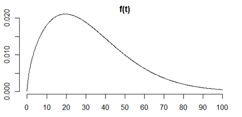
This is a simple distribution of survival probabilities across age. It could be survival of a battery after manufacture, a person after a diagnosis, or a bout of unemployment.
It is unrepresentative, but easy to work with. For anyone who is curious, this curve represents a Weibull distribution with a shape parameter of 1.6 and a scale parameter of 36.
The curve is the probability density function, a commonly used function where areas under the curve represent probabilities of falling within a particular interval.
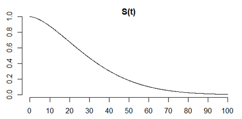
This is the survival function, or the complement of the cumulative distribution function. The Y-axis here is the proportion of the sample who is still alive. The X axis is age.
It starts at 1 because everyone is alive at time zero, and gradually declines to zero, because no one is immortal.
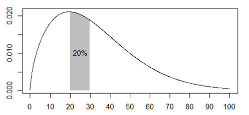
Here is a plot that shows that the probability of death between the ages of 20 and 30 is about 1 in 5.
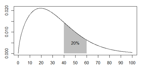
This plot shows that the probability of death between the ages of 40 and 60 is also about 1 in 5.
Apples to oranges comparison
Although the two probabilities are equal, the comparison is not a “fair” comparison. The first event, dying between 20 and 30 years of age, is an apple and the second, dying between 40 and 60 years of age is an orange.
There are three problems with trying to compare these events.
- The number of people alive at age 20 is much larger than the number of people alive at age 40.
- The probabilities are measured across different time ranges.
- The probabilities are quite heterogenous across the time intervals.
A fairer comparison–the hazard function.
The hazard function fixes the three problems noted above.
- It adjusts for the fact that fewer people are alive at age 40 than at age 20.
- It calculates a rate by dividing by the time range.
- It calculates the rate over a narrow time interval, .
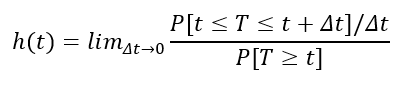
Here’s the mathematical definition.
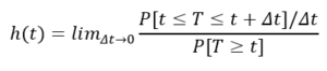
Let’s pull this apart piece by piece.
The denominator,  , is an adjustment for the number of people still alive at time t.
The numerator, 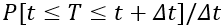 , is a rate and not a probability because we divide by the width of the interval.
The limit,  , insures that the calculation is done over a narrow time interval.
The limit may remind you of formulas you’ve seen for the derivative in your Calculus class (if you took Calculus). If you remember those days of long ago, you may be able to show that
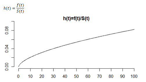
This is what the survival function looks like for our particular example. The hazard function here is much less than one, but it can be bigger than one because it is not a probability. Think of the hazard as a short term measure of risk. In this example, the risk is higher as age increases.
Why is the hazard function important?
The shape of the hazard function tells you some important qualitative information about survival. There are four general patterns worth noting.
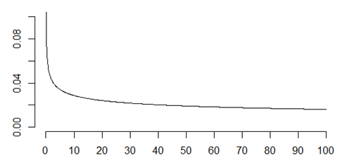
Monotone increasing hazard function
The hazard function shown above is an example of a monotone increasing hazard. The short-term risk of death at 20, given that you survived until your 20th birthday, is about 0.031. But at the age of 40, your hazard function is 0.047.
That means that your short-term risk of death given that you survived until your 40th birthday is worse. The advertising phrase, “You’re not getting older, you’re getting better” doesn’t really apply.
You’ve done well to make it this far, but your short term prospects are grimmer than they were at 20, and things will continue to go downhill. This is why life insurance costs more as you get older.
In a manufacturing setting a monotone increasing hazard function means that new is better than used. This is true for automobiles, for example, which is why if I wanted to trade in my 2008 Prius for a 2020 model, I’d have to part with at least $20,000 dollars.
Batteries also follow a monotone increasing hazard. I have four smoke alarms in my house and the batteries always seem to fail at 3am, necessitating a late night trip to get a replacement. If I was smart, I’d have a stock of extra batteries in hand.
But another strategy would be that when one battery fails at 3am, I should replace not just that battery, but the ones in the other three smoke alarms at the same time.
The short term risk is high for all batteries so I would be throwing away three batteries that were probably also approaching the end of their lifetime, and I’d save myself from more 3am failures in the near future.
Monotone decreasing hazard function
Not everything deteriorates over time. Many electronic systems tend to get stronger over time. The short term risk of failure is high early in the life of some electronic systems, but that risk goes down over time.
The longer these systems survive without failure, the tougher they become. This evokes the famous saying of Friedrich Nietzsche, “That which does not kill us, makes us stronger.”
Many manufacturers will use a monotone decreasing hazard function to their advantage. Before shipping electronic systems with a decreasing hazard function, the manufacturer will run the system for 48 hours.
Better for it to fail on the factory floor where it is easily swapped out for another system. The systems that do get shipped after 48 are tougher and more reliable than ones fresh off the factory floor, leading to a savings in warranty expenses.
A monotone decreasing hazard means that used is better than new. Products with a decreasing hazard almost always are worth more over time than new products. Think of them as being “battle hardened.”
Constant hazard function
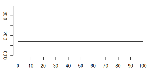
In some settings, the hazard function is constant. This is a situation where new and used are equal. Every product fails over time, but the short term risk of failure is the same at any age. The rate at which radioactive elements decay is characterized by a constant hazard function.
Radon is a difficult gas to work with because every day about 17% of it disappears through radioactive decay.
After two weeks, only 7% of the radon is left. But the 7% that remains has the same rate of disappearance as brand new radon. Atoms don’t show any effects, positive or negative, of age.
Bathtub hazard function
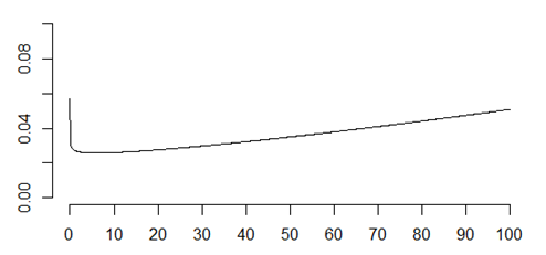
Getting back from machines to humans, your hazard function is a mixture of early decreasing hazard and late increasing hazard. That’s often described as a “bathtub” hazard because the hazard function looks like the side profile of a bathtub with a steep drop on one end and a gradual rise to the other end.
A bathtub hazard recognizes that the riskiest day of your life was the day you were born. If you survived that, the riskiest month of your life was your first month. After that things start to settle down.
But gradually, as parts of your body tend to wear out, the short term risk increases again and if you live to a ripe old age of 90, your short term risk might be as bad as it was during your first year of life.
Most of us won’t live that long but the frailty of an infant and the frailty of a 90 year old are comparable, but for different reasons. The things that kill an infant are different than the things that kill an old person.
I’m not an actuary, so I apologize if some of my characterizations of risk over age are not perfectly accurate. I did try to match up my numbers roughly with what I found on the Internet, but I know that this is, at best, a crude approximation.
Proportional hazards models
The other reason that hazard functions are important is that they are useful in developing statistical models of survival.
The general shape of the hazard function–monotone increasing, monotone decreasing, bathtub–doesn’t change from one group of patients to another. But often the hazard of one group is proportionately larger or smaller than the others.
If this proportionality in hazard functions applies, then the mathematical details of the statistical models are greatly simplified.
It doesn’t always have to be this way. When you are comparing two groups of patients, one getting a surgical treatment for their disease and another getting a medical treatment, the general shapes might be quite different.
Surgery might have a decreasing hazard function. The risks of surgery (infection, excessive bleeding) are most likely to appear early and the longer you stay healthy, the less the risk that the surgery will kill you.
The risks of drugs, on the other hand, might lead to an increasing hazard function. The cumulative dosages over time might lead to greater risk the longer you are on the drugs.
This doesn’t always happen, but when you have different shapes for the hazard function depending on what treatment you are getting, the analysis can still be done, but it requires more effort.
You can’t assume that the hazards are proportional in this case and you have to account for this with a more complex statistical model.
Summary
The hazard function is a short term measure of risk that accounts for the fact your risk of death changes as you age. The shape of the hazard function has important ramifications in manufacturing.
When you can assume that the hazard functions are proportional between one group of patients and another, then your statistical models are greatly simplified.
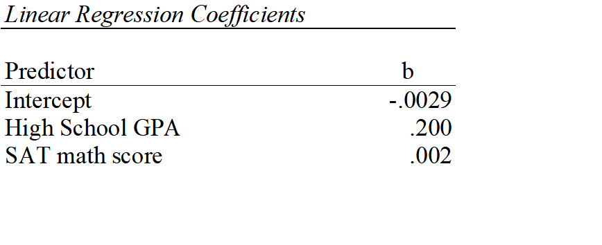 Let’s interpret those coefficients.