data

Free May Craft of Statistical Analysis Webinar: Unlocking the Power of Stata’s Macros and Loops

There are many steps to analyzing a dataset. One of the first steps is to create tables and graphs of your variables in order to understand what is behind the thousands of numbers on your screen. But the type of table and graph you create depends upon the type of variable you are looking at.

There certainly isn’t much point in running a frequency table for a continuous variable with hundreds of unique observations. Creating a boxplot to look for outliers doesn’t make much sense if the variable is categorical. Creating a histogram for a dummy variable would be senseless as well.

How should you start this process? Should you create a spreadsheet listing all the names of the variables and list what type of variable they are? Should you paste the names into a Word document?

In this free webinar with Stata expert Jeff Meyer, you will discover the code to quickly determine the type of every variable in a dataset. By simply pressing the execute button on a do-file you will observe Stata placing each variable in a group (the macro) based on the type of variable it is.

You will watch, through the use of loops, Stata create the proper table and graph for each type of variable in a matter of minutes and output the data into a pdf file for future viewing. You will also receive the code to recreate and practice what you’ve learned.

Title: Improving Your Productivity by Unlocking the Power of Stata’s Macros and Loops
Date: Thurs, May 26, 2016
Time: 1-2 pm EDT
Presenter: Jeff Meyer

This webinar has already taken place. Please sign up below to get access to the video recording.

Statistically Speaking members can access this recording from the Analysis Toolbox Resources page at the Programs Center without signing up.

Jeff Meyer is a statistical consultant with The Analysis Factor, a stats mentor for Statistically Speaking membership, and a workshop instructor. Read more about Jeff here.

Member Training: Communicating Statistical Results: When to Use Tables vs Graphs to Tell the Data’s Story

by guest 2 Comments

In this webinar, we’ll discuss when tables and graphs are (and are not) appropriate and how people engage with each of these media.

Then we’ll discuss design principles for good tables and graphs and review examples that meet these principles. Finally, we’ll show that the choice between tables and graphs is not always dichotomous: tables can be incorporated into graphs and vice versa.

Participants will learn how to bring more thoughtfulness to the process of deciding when to use tables and when to use graphs in their work. They will also learn about design principles and examples they can adopt to create better tables and graphs.

Note: This training is an exclusive benefit to members of the Statistically Speaking Membership Program and part of the Stat’s Amore Trainings Series. Each Stat’s Amore Training is approximately 90 minutes long.

R is Not So Hard! A Tutorial, Part 20: Useful Commands for Exploring Data

by guest 2 Comments

by David Lillis, Ph.D.

Sometimes when you’re learning a new stat software package, the most frustrating part is not knowing how to do very basic things. This is especially frustrating if you already know how to do them in some other software.

Let’s look at some basic but very useful commands that are available in R.

We will use the following data set of tourists from different nations, their gender and numbers of children. Copy and paste the following array into R.

A <- structure(list(NATION = structure(c(3L, 3L, 3L, 1L, 3L, 2L, 3L,
1L, 3L, 3L, 1L, 2L, 2L, 3L, 3L, 3L, 2L), .Label = c("CHINA",
"GERMANY", "FRANCE"), class = "factor"), GENDER = structure(c(1L,
2L, 2L, 1L, 2L, 1L, 2L, 1L, 2L, 2L, 1L, 1L, 1L, 1L, 2L, 1L, 1L
), .Label = c("F", "M"), class = "factor"), CHILDREN = c(1L,
3L, 2L, 2L, 3L, 1L, 0L, 1L, 0L, 1L, 2L, 2L, 1L, 1L, 1L, 0L, 2L
<)), .Names = c("NATION", "GENDER", "CHILDREN"), row.names = 2:18, class = "data.frame")

Want to check that R read the variables correctly? We can look at the first 3 rows using the head() command, as follows:

head(A, 3)
  NATION   GENDER   CHILDREN
2 FRANCE      F        1
3 FRANCE      M        3
4 FRANCE      M        2

Now we look at the last 4 rows using the tail() command:

tail(A, 4)
    NATION   GENDER  CHILDREN
15  FRANCE      F        1
16  FRANCE      M        1
17  FRANCE      F        0
18 GERMANY      F        2

Now we find the number of rows and number of columns using nrow() and ncol().

nrow(A)
[1] 17

ncol(A)
[1] 3

So we have 17 rows (cases) and three columns (variables). These functions look very basic, but they turn out to be very useful if you want to write R-based software to analyse data sets of different dimensions.

Now let’s attach A and check for the existence of particular data.

attach(A)

As you may know, attaching a data object makes it possible to refer to any variable by name, without having to specify the data object which contains that variable.

Does the USA appear in the NATION variable? We use the any() command and put USA inside quotation marks.

any(NATION == "USA")
[1] FALSE

Clearly, we do not have any data pertaining to the USA.

What are the values of the variable NATION?

levels(NATION)
[1] "CHINA"   "GERMANY" "FRANCE"

How many non-missing observations do we have in the variable NATION?

length(NATION)
[1] 17

OK, but how many different values of NATION do we have?

length(levels(NATION))
[1] 3

We have three different values.

Do we have tourists with more than three children? We use the any() command to find out.

any(CHILDREN > 3)
[1] FALSE

None of the tourists in this data set have more than three children.

Do we have any missing data in this data set?

In R, missing data is indicated in the data set with NA.

any(is.na(A))
[1] FALSE

We have no missing data here.

Which observations involve FRANCE? We use the which() command to identify the relevant indices, counting column-wise.

which(A == "FRANCE")
[1]  1  2  3  5  7  9 10 14 15 16

How many observations involve FRANCE? We wrap the above syntax inside the length() command to perform this calculation.

length(which(A == "FRANCE"))
[1] 10

We have a total of ten such observations.

That wasn’t so hard! In our next post we will look at further analytic techniques in R.

*****

See our full R Tutorial Series and other blog posts regarding R programming.

About the Author: David Lillis has taught R to many researchers and statisticians. His company, Sigma Statistics and Research Limited, provides both on-line instruction and face-to-face workshops on R, and coding services in R. David holds a doctorate in applied statistics.

Member Training: A Gentle Introduction to Bayesian Data Analysis

by guest Leave a Comment

P-values are the fundamental tools used in most inferential data analyses [Read more…] about Member Training: A Gentle Introduction to Bayesian Data Analysis

3 Tips for Keeping Track of Data Files in a Large Data Analysis

by Karen Grace-Martin Leave a Comment

If you’ve ever worked on a large data analysis project, you know that just keeping track of everything is a battle in itself.

Every data analysis project is unique and there are always many good ways to keep your data organized.

In case it’s helpful, here are a few strategies I used in a recent project that you may find helpful. They didn’t make the project easy, but they helped keep it from spiraling into overwhelm.

1. Use file directory structures to keep relevant files together

In our data set, it was clear which analyses were needed for each outcome. Therefore, all files and corresponding file directories were organized by outcomes.

Organizing everything by outcome variable also allowed us to keep the unique raw and cleaned data, programs, and output in a single directory.

This made it always easy to find the final data set, analysis, or output for any particular analysis.

You may not want to organize your directories by outcome. Pick a directory structure that makes it easy to find each set of analyses with corresponding data and output files.

2. Split large data sets into smaller relevant ones

In this particular analysis, there were about a dozen outcomes, each of which was a scale. In other words, each one had many, many variables.

Rather than create one enormous and unmanageable data set, each outcome scale made up a unique data set. Variables that were common to all analyses–demographics, controls, and condition variables–were in their own data set.

For each analysis, we merged the common variables data set with the relevant unique variable data set.

This allowed us to run each analysis without the clutter of irrelevant variables.

This strategy can be particularly helpful when you are running secondary data analysis on a large data set.

Spend some time thinking about which variables are common to all analyses and which are unique to a single model.

3. Do all data manipulation in syntax

I can’t emphasize this one enough.

As you’re cleaning data it’s tempting to make changes in menus without documenting them, then save the changes in a separate data file.

It may be quicker in the short term, but it will ultimately cost you time and a whole lot of frustration.

Above and beyond the inability to find your mistakes (we all make mistakes) and document changes, the problem is this: you won’t be able to clean a large data set in one sitting.

So at each sitting, you have to save the data to keep changes. You don’t feel comfortable overwriting the data, so instead you create a new version.

Do this each time you clean data and you end up with dozens of versions of the same data.

A few strategic versions can make sense if each is used for specific analyses. But if you have too many, it gets incredibly confusing which version of each variable is where.

Picture this instead.

Start with one raw data set.

Write a syntax file that opens that raw data set, cleans, recodes, and computes new variables, then saves a finished one, ready for analysis.

If you don’t get the syntax file done in one sitting, no problem. You can add to it later and rerun everything from your previous sitting with one click.

If you love using menus instead of writing syntax, still no problem.

Paste the commands as you go along. The goal is not to create a new version of the data set, but to create a clean syntax file that creates the new version of the data set. Edit it as you go.

If you made a mistake in recoding something, edit the syntax, not the data file.

Need to make small changes? If it’s set up well, rerunning it only takes seconds.

There is no problem with overwriting the finished data set because all the changes are documented in the syntax file.

Preparing Data for Analysis is (more than) Half the Battle

by Karen Grace-Martin 2 Comments

Just last week, a colleague mentioned that while he does a lot of study design these days, he no longer does much data analysis.

His main reason was that 80% of the work in data analysis is preparing the data for analysis. Data preparation is s-l-o-w and he found that few colleagues and clients understood this.

Consequently, he was running into expectations that he should analyze a raw data set in an hour or so.

You know, by clicking a few buttons.

I see this as well with clients new to data analysis. While they know it will take longer than an hour, they still have unrealistic expectations about how long it takes.

So I am here to tell you, the time-consuming part is preparing the data. Weeks or months is a realistic time frame. Hours is not.

(Feel free to send this to your colleagues who want instant results).

There are three parts to preparing data: cleaning it, creating necessary variables, and formatting all variables.

Data Cleaning

Data cleaning means finding and eliminating errors in the data. How you approach it depends on how large the data set is, but the kinds of things you’re looking for are:

Impossible or otherwise incorrect values for specific variables
Cases in the data who met exclusion criteria and shouldn’t be in the study
Duplicate cases
Missing data and outliers
Skip-pattern or logic breakdowns
Making sure that the same value of string variables is always written the same way (male ≠ Male in most statistical software).

You can’t avoid data cleaning and it always takes a while, but there are ways to make it more efficient.

For example, one way to find impossible values for a variable is to print out data for cases outside a normal range.

This is where learning how to code in your statistical software of choice really helps. You’ll need to subset your data using IF statements to find those impossible values.

But if your data set is anything but small, you can also save yourself a lot of time, code, and errors by incorporating efficiencies like loops and macros so that you can perform some of these checks on many variables at once.

Creating New Variables

Once the data are free of errors, you need to set up the variables that will directly answer your research questions.

It’s a rare data set in which every variable you need is measured directly.

So you may need to do a lot of recoding and computing of variables.

Examples include:

Creating change scores
Creating indices from scales
Combining too-small-to-use categories of nominal variables
Centering variables
Restructuring data from wide format to long (or the reverse)

And of course, part of creating each new variable is double-checking that it worked correctly.

Formatting Variables

Both original and newly created variables need to be formatted correctly for two reasons:

First, so your software works with them correctly. Failing to format a missing value code or a dummy variable correctly will have major consequences for your data analysis.

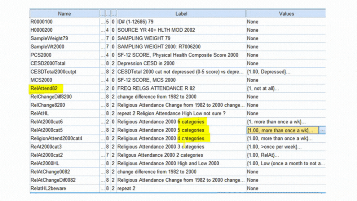
Second, it’s much faster to run the analyses and interpret results if you don’t have to keep looking up which variable Q156 is.

Examples include:

Setting all missing data codes so missing data are treated as such
Formatting date variables as dates, numerical variables as numbers, etc.
Labeling all variables and categorical values so you don’t have to keep looking them up.

All three of these steps require a solid knowledge of how to manage data in your statistical software. Each one approaches them a little differently.

It’s also very important to keep track of and be able to easily redo all your steps. Always assume you’ll have to redo something. So use (or record) syntax, not menus.