There are many statistical concepts that are easy to confuse.
Sometimes the problem is the terminology. We have a whole series of articles on Confusing Statistical Terms.
But in these cases, it’s the concepts themselves. Similar, but distinct concepts that are easy to confuse.
Some of these are quite high-level, and others are fundamental. For each article, I’ve noted the Stage of Statistical Skill at which you’d encounter it.
So in this series of articles, I hope to disentangle some of those similar, but distinct concepts in an intuitive way.
Stage 1 Statistical Concepts
The Difference Between:
Stage 2 Statistical Concepts
The Difference Between:
Stage 3 Statistical Concepts
The Difference Between:
Are there concepts you get mixed up? Please leave it in the comments and I’ll add to my list.
What does it mean for two variables to be correlated?
Is that the same or different than if they’re associated or related?
This is the kind of question that can feel silly, but shouldn’t. It’s just a reflection of the confusing terminology used in statistics. In this case, the technical statistical term looks like, but is not exactly the same as, the way we mean it in everyday English. (more…)
Mixed models are hard.
They’re abstract, they’re a little weird, and there is not a common vocabulary or notation for them.
But they’re also extremely important to understand because many data sets require their use.
Repeated measures ANOVA has too many limitations. It just doesn’t cut it any more.
One of the most difficult parts of fitting mixed models is figuring out which random effects to include in a model. And that’s hard to do if you don’t really understand what a random effect is or how it differs from a fixed effect. (more…)
Generalized linear models—and generalized linear mixed models—are called generalized linear because they connect a model’s outcome to its predictors in a linear way. The function used to make this connection is called a link function. Link functions sounds like an exotic term, but they’re actually much simpler than they sound.
For example, Poisson regression (commonly used for outcomes that are counts) makes use of a natural log link function as follows:
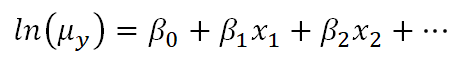
Clearly, there is not a direct linear relationship of the x variables to the average count, but there is a “sort of linear” relationship happening: a function of the mean of y is related to a linear combination of x variables. In other words, the linear model has now been generalized to a bigger type of situation.
This can lead to confusion, though, because on the surface it looks very similar to what happens when we transform the dependent variable in a linear model, like a linear regression.
The key thing to understand is that the natural log link function is a function of the mean of y, not the y values themselves.
Transformations of Y
Below is a linear model equation where the original dependent variable, y, has been natural log transformed. That is, the natural log has been taken of each individual value of y, and that is being used as the dependent variable.
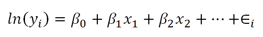
The linear model with the log transformation is providing an equation for an individual value of ln(y). We could also write it as follows, where we are modeling the mean of ln(y) (note the error term is no longer present):
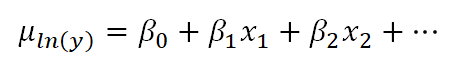
This makes the difference a bit clearer. When we transform the data in a linear model, we are no longer claiming that y is normally distributed around a mean, given the x values — we are claiming that our new outcome variable, ln(yi), is normally distributed.
In fact, we often make this transformation specifically because the values of y do not appear to be normally distributed around their average.
In the case of the Poisson model, however, the link function does not change the distribution of the actual observations in some way to make them something other than Poisson distributed. Instead, the link function defines the relationship of the x variables directly to the mean of the Poisson distributed y. The individual observations then vary around this expected value accordingly.
The mean of the log is not the log of the mean
As you may know, if you have used this kind of data transformation in a linear model before, you cannot simply take the exponent of the mean of ln(y) to get the mean of y.
You might be surprised to know, though, that you can do this with a link function. If you have specific values of your x variables, you can calculate the predicted average count, μy based on those x values by inversing the natural log:
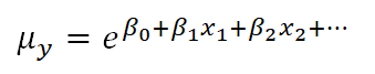
This ability to back-transform means (and regression coefficients) to a more intuitive scale is part of what makes generalized linear models so useful.
Go to the next article or see the full series on Easy-to-Confuse Statistical Concepts
One question that seems to come up pretty often is:
What is the difference between logistic and probit regression?
Well, let’s start with how they’re the same:
Both are types of generalized linear models. This means they have this form:

(more…)
One of the many confusing issues in statistics is the confusion between Principal Component Analysis (PCA) and Factor Analysis (FA).
They are very similar in many ways, so it’s not hard to see why they’re so often confused. They appear to be different varieties of the same analysis rather than two different methods. Yet there is a fundamental difference between them that has huge effects on how to use them.
(Like donkeys and zebras. They seem to differ only by color until you try to ride one).
Both are data reduction techniques—they allow you to capture the variance in variables in a smaller set.
Both are usually run in stat software using the same procedure, and the output looks pretty much the same.
The steps you take to run them are the same—extraction, interpretation, rotation, choosing the number of factors or components.
Despite all these similarities, there is a fundamental difference between them: PCA is a linear combination of variables; Factor Analysis is a measurement model of a latent variable.
Principal Component Analysis
PCA’s approach to data reduction is to create one or more index variables from a larger set of measured variables. It does this using a linear combination (basically a weighted average) of a set of variables. The created index variables are called components.
The whole point of the PCA is to figure out how to do this in an optimal way: the optimal number of components, the optimal choice of measured variables for each component, and the optimal weights.
The picture below shows what a PCA is doing to combine 4 measured (Y) variables into a single component, C. You can see from the direction of the arrows that the Y variables contribute to the component variable. The weights allow this combination to emphasize some Y variables more than others.
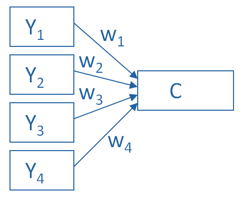
This model can be set up as a simple equation:
C = w1(Y1) + w2(Y2) + w3(Y3) + w4(Y4)
Factor Analysis
A Factor Analysis approaches data reduction in a fundamentally different way. It is a model of the measurement of a latent variable. This latent variable cannot be directly measured with a single variable (think: intelligence, social anxiety, soil health). Instead, it is seen through the relationships it causes in a set of Y variables.
For example, we may not be able to directly measure social anxiety. But we can measure whether social anxiety is high or low with a set of variables like “I am uncomfortable in large groups” and “I get nervous talking with strangers.” People with high social anxiety will give similar high responses to these variables because of their high social anxiety. Likewise, people with low social anxiety will give similar low responses to these variables because of their low social anxiety.
The measurement model for a simple, one-factor model looks like the diagram below. It’s counter intuitive, but F, the latent Factor, is causing the responses on the four measured Y variables. So the arrows go in the opposite direction from PCA. Just like in PCA, the relationships between F and each Y are weighted, and the factor analysis is figuring out the optimal weights.
In this model we have is a set of error terms. These are designated by the u’s. This is the variance in each Y that is unexplained by the factor.
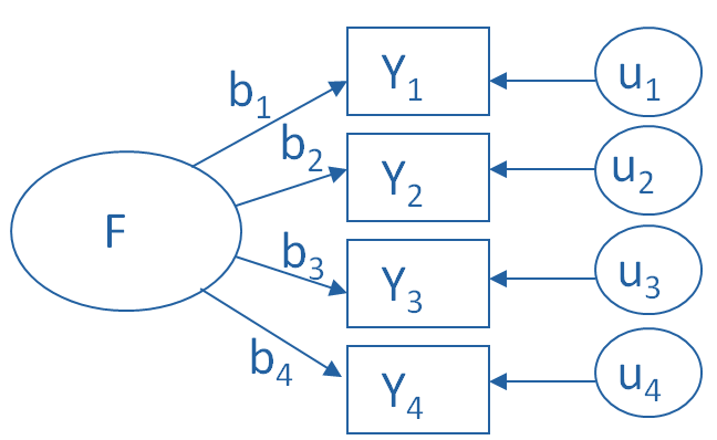
You can literally interpret this model as a set of regression equations:
Y1 = b1*F + u1
Y2 = b2*F + u2
Y3 = b3*F + u3
Y4 = b4*F + u4
As you can probably guess, this fundamental difference has many, many implications. These are important to understand if you’re ever deciding which approach to use in a specific situation.
Go to the next article or see the full series on Easy-to-Confuse Statistical Concepts